
The Age of Incognito
Published:
Overview
The following project was the output for the final project requirement in our Big Data and Cloud Computing class for MSc in Data Science. The challenge for the project was in the context of the increasing need for data privacy in online transactions and activities. This project was presented to the public during the Big Data Presentations held in Asian Institute of Management on December 5, 2019. This report contains some explicit language pertaining to adult videos. For a censored version, see the pdf report below.
Acknowledgements
This project was done with my teammates Criselle David, Gem Gloria, and Janlo Cordero.
PDF Report
You may also view a PDF version of this report. I'd recommend going through the presentation deck if you want a more visual overview of the methodology and results that we garnered. In this case, the PDF is also censored for explicit terms.
The presentation is available here: pdf
The Age of Incognito: Utilizing Big D in the Adult Film Industry
Carlo Angelo Z. Cordero, Criselle Angela M. David, Gemille Isabel Gloria, Kyle Mathew P. Ong
MSDS 2020
1 Executive Summary
In the age of data privacy concerns, especially after the Facebook-Cambridge Analytica scandal, recommender systems of online platforms are continuously threatened to be cut-off from their leverage: user level transactional data. The rich digital footprint that we leave by using the internet is used to serve us hyper-targeted ads and relevant content by digital marketers and streaming platforms such as Netflix, Spotify and Amazon. But without these data, most recommender system engines would fail and the age of Watch Next and Daily Mix that we know off would cease to exist.
In this study, we explore building a recommender system which does not depend on user level transactional data. Our content-based recommender system is based on aggregate viewer preferences using video views and video content aware tags. Our dataset is composed of 6.8 million video metadata from Pornhub consisting of uploads from 2007 to November 2019. The system aims to address three important facets: a balance between the diversity and similarity of recommended content, and the past behavior of users by using implicit ratings through aggregate views. To achieve this, we use association rule mining to uncover which set of tags the user might like given that he or she is watching a video with a certain set of tags. Clustering was used to control the similarity of recommendations and to ensure that recommended videos are not too far off from each other, content-wise.
Evaluation of the recommendations show that there are certain tags that produce homogenous recommendations, meaning, the recommended videos tend to remain in the same cluster. These tags can be qualitatively categorized as fetishes. Other more general tags tend to lead to more diverse recommendations.
A more quantitative analysis of the recommendations is highly advised although this entails either collection of user specific data or deployment of the model, both of which are outside the scope of study.
2 Introduction
In 2018, Cambridge Analytica, a political consulting firm known to leverage digital assets to launch campaigns, was revealed to have harvested personal data from millions of Facebook users without consent and used it for political advertising. This caused a massive outcry meriting a congress hearing where Mark Zuckerberg, Facebook founder and CEO, testified. Due to this scandal, issues of data privacy, data breach, and identity theft has been brought forth into public consciousness.
With the advent of social media, an increasing volume of personal information is being collected. According to research, users control of 70% of their digital footprint by consciously maintaining a personal digital footprint strategy, which includes choosing which details to share on social media. However, the remaining 30% are uncontrolled streams of dynamic digital signatures which have been used in cases of data breach and identity theft. [1]
Services like Netflix, Amazon, and Spotify rely heavily on tracking user data in order to serve content. User-based collaborative filtering, one of the most popular and widely used recommender systems, tracks user activity history in order to generate future recommendations. Other more advanced systems include tracking browsing history, past purchases, location, and even chat logs to increase engagement and conversion rates.
Current proposals for privacy protection laws including a strict enforcement of ‘do not track’ user requests, and purging of session data after exit [2] would severely limit the data collection of the previously mentioned sites and would hamper the performance of existing recommender systems. Studies have explored several methodologies that excludes user data collection by employing natural language processing or by treating it as a cold-start problem, where there is no available user preference data. [3], [4]
In this study, we explore the use of content-based recommender system by using association rule mining and clustering to serve coherent recommendations without relying on tracking user data. This is done using the Pornhub dataset containing only video metadata including tags, number of views and ratings. The system aims to address three important facets: a balance between the diversity and similarity of recommended content, and the past behavior of users by using implicit ratings through aggregate views.
3 Data Description
Data Description The original dataset consists of 25GB worth of html metadata of all Pornhub videos at the time of download. The following information were extracted from the metadata:
- Title
- Upload date
- Video duration
- Views
- Upvotes
- Downvotes
- Tags
- Categories
In total, there are around 6.8 million videos with an aggregate of 304 billion views spanning from 2007 to November 2019. The dataset (updated daily) can be directly downloaded from this <a href=https://www.pornhub.com/pornhub.com-db.zip>link</a>.
# Standard Imports
import pandas as pd
import numpy as np
import matplotlib.pyplot as plt
%matplotlib inline
import glob
import seaborn as sns
from time import time
import pickle
from IPython.display import clear_output
from collections import Counter

# Machine Learning Imports
from sklearn.feature_extraction.text import CountVectorizer
from sklearn.decomposition import TruncatedSVD
from scipy.spatial.distance import euclidean, cityblock
from sklearn.manifold import TSNE
from sklearn.preprocessing import MinMaxScaler, StandardScaler, RobustScaler
from sklearn.decomposition import TruncatedSVD
from sklearn.cluster import Birch as Birch
from sklearn.metrics.pairwise import cosine_similarity

# Dask Imports
import dask
from dask.diagnostics import ProgressBar
pbar = ProgressBar()
pbar.register()
from dask.distributed import Client
import dask.dataframe as dd
import dask.array as da
import dask.bag as dbag
from dask import delayed
from dask_ml.feature_extraction.text import HashingVectorizer
from dask_ml.cluster import KMeans
# from dask_ml.decomposition import TruncatedSVD
4 Methodology
Our methodology for this project consists of five parts:
- Preprocessing
- Exploratory Data Analysis
- Association Rule Mining
- Clustering
- Aggregation (Recommender System)
Each part is explained in their respective sections below.
In general, we use the same algorithm behind user-based collaborative filtering where we have three main features: users, items and ratings. Since our dataset does not have user level transactions, we substitute videos per user and items as tags and use views as implicit ratings. The goal is to provide the user watching a certain video a recommendation of the next video to watch using the inherent features of video such as tags and aggregate views.
4.1 Preprocessing
The raw file is a csv which contains one html iframe per line. In order to process this into a more manageable format, we load the file into a dask bag use regex to parse the following information from the metadata:
- Title
- Upload date
- Video duration
- Views
- Upvotes
- Downvotes
- Tags
- Categories
The resulting file is 2.0GB of json which can be loaded in either a distributed dataframe or pandas dataframe depending on the need. Titles were label encoded in the interest of limiting storage size. The preprocessing notebook can be found here.
4.2 Exploratory Data Analysis
Our initial EDA shows that the video metadata collected ranges from 2007 to the date of collection in November 2019, with the number of videos posted growing exponentially in the recent years.
<img src=/images/incognito-recommender/vidperyear.png>
The length of videos and number of views are also logarithmically distributed:
<img src=/images/incognito-recommender/length.png>
The bulk of videos have around 10,000 views with outliers that reach 100 million views. These videos are in the 99th percentile of views. <img src=/images/incognito-recommender/views.png>
For tags, there are more than 300,000 unique tags ranging from broad video categories to very specific ones. The average video has 5 tags, which we will use later as basis for the number of tags for our recommender system.
EDA notebook can be found <a href=EDA.ipynb>here.</a>
4.3 Association Rule Mining
PySpark’s frequent itemset mining implementation uses the FPGrowth algorithm. FPGrowth builds a vertical database and passes through the entire transactional database once for efficiency and then builds frequent item sets by employing the propoerties of frequent itemsets, namely, a frequent itemset with items A and B with transactions $set(tid)_A$ and $set(tid)_B$ respectively, would have an absolute support represented by $n(set(tid)_A \cap set(tid)_B)$.
After frequent itemset mining, we build association rules by using the supports of the itemsets to build a list of antecedents and their corresponding consuquents. The idea is a user is most likely to purchase item B given that he or she has purchased item A, a relationship that has been implied given our large transactional database.
We utilize each video as a transaction and the associated tags as items. The resulting frequent itemset is a set of most commonly associated tags found in each video. We export the resulting rules with the corresponding antecedent and consequents for further integration with our main recommender system.
The figure below shows the raw input to the fpgrowth function:
<img src=/images/incognito-recommender/transactional_db.png>
After frequent set mining, the resulting dataframe consists of the antecedent and consequents as show below:
<img src=/images/incognito-recommender/rules.png>
The complete notebook used for this part can be found here.
4.4 Clustering
Unsupervised clustering helps extract information on inherent groupings within the dataset. After generating the association rules for the itemset of tags, the entire corpus of videos is then clustered in order to find the similar video groups within the dataset. This will help in verifying and understanding how the recommender system generates new recommendations; that is, if the generated recommendations show a certain pattern in its recommendations per group/cluster. The clustering method is broken down into 4 phases:
- Bag of Words Representation
- Dimensionality Reduction and Scaling
- KMeans Clustering
- Evaluation and Interpretation
4.4.1 Bag of Words Representation
As the main features of each video in the dataset is the tags associated with the video, these words are converted into a bag of words representation that show all the possible tags within the dataset. To facilitate this, we implement the CountVectorizer package on python which converts the words into vector representations for the entire dataset. On most natural language processing tasks, the Term-Frequency Inverse Document Frequency (TFIDF) is preferred as this puts a weight on each term/word that is more representative of the importance of such words in natural language. However, in this case, as the words are not representative of words in a sentence but rather a set of tags that describe each video, the count vectorizer method is preferred. In order to limit the number of terms, a min_df of 0.002 is set and max_features of 1000.
df = pd.read_pickle('criselle/df_clean.pkl')
CV = CountVectorizer(min_df=.002, max_features=1000)
CV.fit(df['tags'])
CountVectorizer(analyzer='word', binary=False, decode_error='strict',
                dtype=<class 'numpy.int64'>, encoding='utf-8', input='content',
                lowercase=True, max_df=1.0, max_features=1000, min_df=0.002,
                ngram_range=(1, 1), preprocessor=None, stop_words=None,
                strip_accents=None, token_pattern='(?u)\\b\\w\\w+\\b',
                tokenizer=None, vocabulary=None)
bow = CV.transform(df['tags'])
bow.shape
(6859483, 496)
4.4.2 Dimiensionality Reduction and Scaling
As we end up with a large amount of features for the bag of words representation, Truncated Singular Value Decomposition (TSVD) is performed on the dataset to limit the features. In this case, the number of latent factors is chosen such that the variance explained of the latent factors is around 60%. After reducing the dimensions of the dataset, the integer features such as length, views, ups, and downs are added to the columns as features. These are also scaled using a MinMaxScaler so that the values will not be orders of magnitude different from the bag of words representation.
df.length = df.length.astype(int)
scaler = MinMaxScaler()
scaled_int = scaler.fit_transform(df[['length', 'views', 'ups', 'downs']])
TSVD = TruncatedSVD(n_components=50, random_state=2020)
TSVD.fit(bow)
TruncatedSVD(algorithm='randomized', n_components=50, n_iter=5,
             random_state=2020, tol=0.0)
newbow = TSVD.transform(bow)
TSVD.explained_variance_ratio_.sum()
0.5914244685608808
newbow.shape
(6859483, 50)
X = np.hstack((newbow, scaled_int))
4.4.3 KMeans Clustering
The clustering algorithm used in this case is KMeans. This is a simple but relatively powerful clustering algorithm that looks at the distance of the different points from a randomly initiated “centroid” point that represents a cluster. The distances are then taken and iteratively shifts the center points to the mean of all of the distances of the points in the original cluster. This is then done until the difference in the position of the cluster centroids converges or does not change anymore.
dabow = da.from_array(X)
dabow
|
km = KMeans(n_clusters=15, random_state=2020, n_jobs=-1)
km.fit(dabow)
km.inertia_
save models for future use
# # save clustering matrix
# with open('../../s3/cluster_X.pkl', 'wb') as f:
#     pickle.dump(X, f)
# # save count vectoriizer, scaler, TSVD, and Kmeans model
# with open('../../s3/cluster_cv_scaler_tsvd_km.pkl', 'wb') as f:
#     pickle.dump((CV, scaler, TSVD, km), f)
# load clustering matrix
with open('criselle/cluster_X.pkl', 'rb') as f:
    X = pickle.load(f)
# load count vectoriizer, scaler, TSVD, and Kmeans model
with open('criselle/cluster_cv_scaler_tsvd_km.pkl', 'rb') as f:
    CV, scaler, TSVD, km = pickle.load(f)
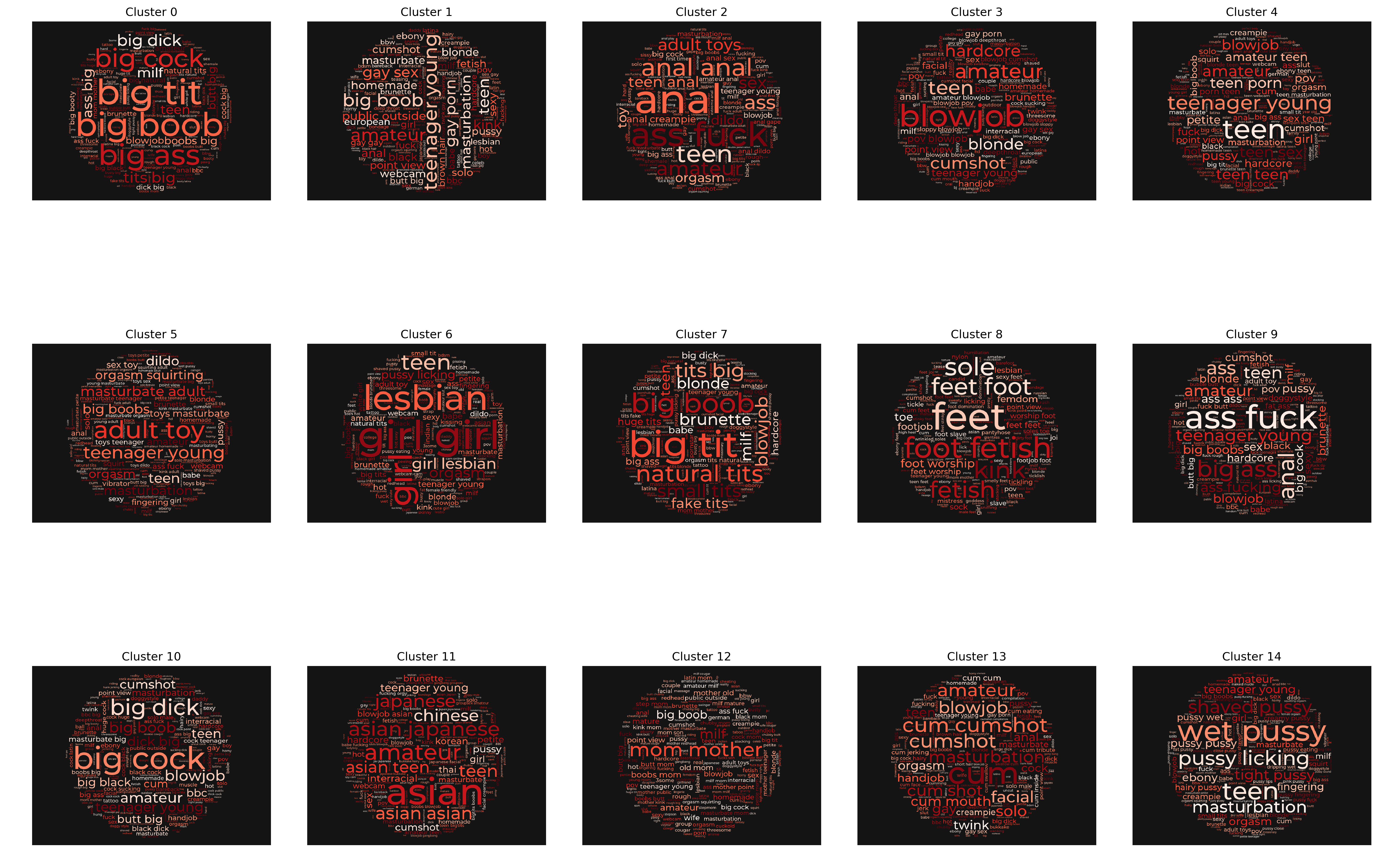
To interpret our clusters, we will look at the wordcloud and number of tags of each cluster. This will help us in determining the defining factors of each cluster. Since KMeans is an unsupervised task, the burden of interpreting the meaning of each cluster lies on the analysis of each cluster. In this case, since the tags are effectively words, we will be relying on the wordcloud of each of the clusters as well as looking at the counts of each tag that appears in each cluster.
clusters = km.labels_.compute()
[########################################] | 100% Completed | 2.9s
if len(df) == len(clusters):
    df['cluster'] = clusters
else:
    print('error, invalid lengths')
df['tagset'] = df['tags'].apply(lambda x: x.split(';'))
# # save cluster summary
# with open('../../s3/cluster_summary.pkl', 'wb') as f:
#     pickle.dump(results, f)
# load cluster summary
with open('criselle/cluster_summary.pkl', 'rb') as f:
    results = pickle.load(f)
res = pd.DataFrame.from_records(results)
res['agg_rating'] = (res['agg_ups'] - res['agg_downs'])/(res['agg_ups']+res['agg_downs'])
for i in range(len(res)):
    print(f'cluster: {i}, {res.iloc[i]["n"]}')
    for j in res.iloc[i]['tags']:
        print(j)
    print(f"views: {res.iloc[i]['views']}\nlength: {res.iloc[i]['length']/60}\nups: {res.iloc[i]['ups']}\ndowns: {res.iloc[i]['downs']}\n\n")
# db = database.compute()
# # save database of tags
# with open('../../s3/tags_db.pkl', 'wb') as f:
#     pickle.dump(db, f)
# load database of tags
with open('criselle/tags_db.pkl', 'rb') as f:
    db = pickle.load(f)
# sample original dataframe by the proportion of each cluster * 1%
sampled = df.groupby('cluster').apply(lambda x: x.sample(n=int(np.floor(len(x)*0.01))))
sampled = sampled.drop('cluster', axis=1).reset_index()
cluster_groups = sampled.groupby('cluster')
tag_words = []
for i in range(15):
    tag_words.append(' '.join(cluster_groups.get_group(i)['tags'].apply(lambda x: ' '.join(x.split(';'))).values))
from wordcloud import WordCloud, STOPWORDS
from PIL import Image
import matplotlib
def plot_wordcloud(clean_string, filename, row=None, col=None, save=False):
    mask = np.array(Image.open("criselle/plot_mask.png"))
    fontpath = 'criselle/Montserrat-Medium.otf'
    wordcloud = WordCloud(font_path=fontpath,
                          background_color="#141414",
                          colormap=matplotlib.cm.Reds,
                          mask=mask,
                          contour_width=0,
                          contour_color='white'
                         ).generate(clean_string)
    return wordcloud
fig, ax = plt.subplots(3,5, dpi=300, figsize=(20,15))
row = 0
col = 0
for i in range(15):
    clear_output()
    print(row, col)
    ax[row,col].imshow(plot_wordcloud(tag_words[i], f'cluster_{i}', row=row, col=col, save=False))
    ax[row,col].axis('off')
    ax[row,col].set_title(f'Cluster {i}')
    col += 1
    if col == 5:
        row += 1
        col = 0
fig.tight_layout()
2 4
list_tags = []
for i in range(15):
    list_tags.append([i[0] for i in Counter(tag_words[i].split(' ')).most_common()])

cluster_tags = pd.DataFrame(list_tags).transpose()
cluster_tags.columns = [f'Cluster {i}' for i in cluster_tags.columns]
cluster_tags.head()
| Cluster 0 | Cluster 1 | Cluster 2 | Cluster 3 | Cluster 4 | Cluster 5 | Cluster 6 | Cluster 7 | Cluster 8 | Cluster 9 | Cluster 10 | Cluster 11 | Cluster 12 | Cluster 13 | Cluster 14 | |
|---|---|---|---|---|---|---|---|---|---|---|---|---|---|---|---|
| 0 | big-boobs | young | ass-fuck | blowjob | teen | adult-toys | girl-on-girl | big-tits | feet | ass-fuck | big-cock | asian | mom | cum | wet-pussy |
| 1 | big-tits | kink | anal | amateur | young | masturbate | lesbian | big-boobs | kink | ass | big-dick | japanese | mother | cumshot | masturbate |
| 2 | big-ass | teenager | young | cumshot | teenager | young | young | blowjob | foot-fetish | big-ass | cumshot | amateur | milf | gay | young |
| 3 | big-cock | gay | adult-toys | teen | teen-sex | teenager | lesbians | brunette | soles | anal | young | teen | big-boobs | masturbation | shaved-pussy |
| 4 | big-dick | amateur | teenager | hardcore | teen-porn | orgasm | teenager | natural-tits | foot-worship | butt | big-boobs | blowjob | old | amateur | pussy |
From the wordcloud and the dataframe of top tags for each cluster, it can be seen that there is a clear distinction between the different clusters. These clusters are then going to be the basis to check whether a recommendation jumps from one cluster, representative of a certain type of video given the tags, to another cluster. We can also take a look at the aggregate statistics of each cluster to determine the:
- most viewed cluster (on average)
- most number of videos
- most liked cluster (on average)
# cluster with most views
res.sort_values('views', ascending=False).head(1)
| views | agg_views | ups | agg_ups | downs | agg_downs | length | tags | n | agg_rating | |
|---|---|---|---|---|---|---|---|---|---|---|
| 6 | 6524.0 | 12471073772 | 26.0 | 34106924 | 6.0 | 11304231 | 480.0 | [(girl-on-girl, 66655), (lesbian, 31092), (you... | 111234 | 0.502139 |
# cluster with most videos
res.sort_values('n', ascending=False).head(1)
| views | agg_views | ups | agg_ups | downs | agg_downs | length | tags | n | agg_rating | |
|---|---|---|---|---|---|---|---|---|---|---|
| 1 | 693.0 | 56827049639 | 6.0 | 168374742 | 1.0 | 52957995 | 257.0 | [(young, 270076), (kink, 261780), (teenager, 2... | 3256823 | 0.521463 |
# most liked cluster
res.sort_values('agg_rating', ascending=False).head(1)
| views | agg_views | ups | agg_ups | downs | agg_downs | length | tags | n | agg_rating | |
|---|---|---|---|---|---|---|---|---|---|---|
| 8 | 1238.0 | 973365945 | 13.0 | 4633177 | 1.0 | 789511 | 304.0 | [(feet, 45239), (kink, 33101), (foot-fetish, 3... | 76665 | 0.708812 |
4.5 Recommender System
To build the recommender system, the results of the association rules and the clustering are both taken into consideration. As the goal is to build a system that will not need to track users’ behavior, the aggregate features of each video is taken into consideration instead. In a traditional user based collaborative filtering approach, the granularity of the data goes down to {user, item} interactions. Using the exampleof the pornhub data, the values of importance to this analysis is the {tags, views} of each video, such that the views of each video already represent the aggregate popularity or preference of the all users for each video. The tags of each video in this framework represents the types of content that belong within the video. This is then indicative of the preference of all users for a certain group of tags. As such, the main methodology uses the views of each video as the total number of “votes” for a particular set of tags.
The results of the association rules applied on the dataset of videos gives us the probability that a user will watch another video given that he/she is currently watching a certain video. In this case, it can already be seen that this algorithm can only work when the user is already currently watching a video. Or, in other words, there needs to be a minimum of at least one interaction/selection by the user for the recommender system to work. This is not exactly the same as the “cold start” problem faced by typical recommender systems as in those scenarios, the system needs to build up a lot of data points on a given user, with the recommendations for each user getting better the more the system collects on their behavior. In the case of the “incognito” recommender system, one interaction is all the system needs since there is no benefit in more interactions from the user as their user-specific behavior will not be tracked.
In building the final recommendation for each user, first the association rules are used to determine a tagset that is most likely going to be watched by a user watching a given video. This is shown as an example below as {current_video_tags} -> {recommended_video_tags}
{'amateur', 'ass', 'babe', 'brunette', 'dancing', 'funny', 'girlfriend', 'teasing', 'webcam'} -> {'butt', 'teen'}
The resulting tag recommendations {'butt', 'teen'} is then a recommendation by the system of a new category or set of categories that would fit the user based on the learned associations. We then take universe of all videos that contain the subset of these tags, and these become our universe of possible recommendations for the user watching a given video.
To further improve the recommendations, we would need to sort these videos and give just the top k number of recommendations. Using the association rules, the algorithm has already determined the “type” of video that is most likely going to be watched by our user. This represents an altogether different set of tags from the original as the association rules remove the original tags by default. To limit and order the recommendations then, we bring back the most similar to the current video being watched using the unsupervised clustering. By doing this, we are essentially using the association rules to recommend a perfectly different category to the current video being watched, but using the unsupervised clustering results to limit these recommendations such that they are not too far or too completely different from the current video. This is done by querying by similarity on the results of the clusters, and ordering the results, the universe of potential recommended videos, by their similarity to the original video. The top k recommendations are then given by the top k most similar videos recommended by the association rules.
def recos(orig, query, top_n=5):

    '''
    Returns the index of the top_n recommendations for a video based on the query of relevant video tags to this video.

    orig : index of original query
    query : list of tags from recommdender system
    '''

    assert isinstance(query, list), "Query must be a list."

    result = db[query]
    query_result = list(set.intersection(*list(result)))

    original_video = X[orig]
    cos_sim = []
    for i in query_result:
        cos_sim.append(cosine_similarity(original_video.reshape(1,-1), X[i].reshape(1,-1))[0,0])

    return np.array(query_result)[np.array(cos_sim).argsort()[::-1]][:top_n]
Since this is a large dataset, we will subset the results by taking 2 randomly sampled videos from each of the 15 original clusters and run the recommender system for each of these.
# load the sample results from association rules EMR
with open('criselle/consequent_sample.pkl', 'rb') as f:
    con = pickle.load(f)
con['len_reco'] = con['recommendations'].apply(lambda x: len(x))
con = con.merge(df.reset_index()[['index', 'title', 'cluster']], left_on='title', right_on='title')
con.index = con['index']
congrp = con.groupby('cluster')
# take the top two (by length of recommendations) tags for each cluster in consequents
qdf = pd.DataFrame()
for i in range(15):
    qdf = qdf.append(congrp.get_group(i).sort_values('len_reco', ascending=False).iloc[:2])
s = time()
qrecos = []
for i in range(len(qdf)):
    clear_output()
    print(f'{i}/{len(qdf)}')
    qrecos.append(recos(qdf.iloc[i].name, qdf['recommendations'].iloc[i]))
e = time()
e - s
29/30


361.5833294391632
# create a dictionary of query_index : [recos index, cluster]
top_recos = dict(zip(qdf.index, zip(qrecos,qdf['cluster'])))
idx = list(top_recos.keys())
# get all the indices of the potential recommendations for all queries
rec_idx = list(set([item for sublist in [i[0] for i in top_recos.values()] for item in sublist]))

# merge all indices
idx = idx + rec_idx
sample_idx = sampled['level_1'].to_list()
sample_idx.extend(idx)
df['tags'] = df['tags'].apply(lambda x: x.split(';'))
s = time()
reco_master = {}
for k,v in top_recos.items():

    recs = df.loc[list(v[0])]

    reco_master[k] = df.loc[k].to_dict()

    reco_master[k]['tx_idx'] = sample_idx.index(k)

    reco_master[k]['recos'] = {}

    for i in range(len(recs)):
        reco_master[k]['recos'][recs.iloc[i].name] = recs.iloc[i].to_dict()
        reco_master[k]['recos'][recs.iloc[i].name]['tx_idx'] = sample_idx.index(recs.iloc[i].name)
e = time()
print(e-s)
2.8898215293884277
# # save reco_master
# with open('../criselle/master_reco_dict.pkl', 'wb') as f:
#     pickle.dump(reco_master, f)
# load the list of all recommendations
with open('criselle/master_reco_dict.pkl', 'rb') as f:
    reco_master = pickle.load(f)
# # save sampled dataframe for plotting
# with open('../criselle/sampled_dataframe_for_plotting.pkl', 'wb') as f:
#     pickle.dump((X[sample_idx], sample_idx), f)
# samplex = X[sample_idx]
# load sample dataframe for plotting
with open('criselle/sampled_dataframe_for_plotting.pkl', 'rb') as f:
    samplex, sample_idx = pickle.load(f)
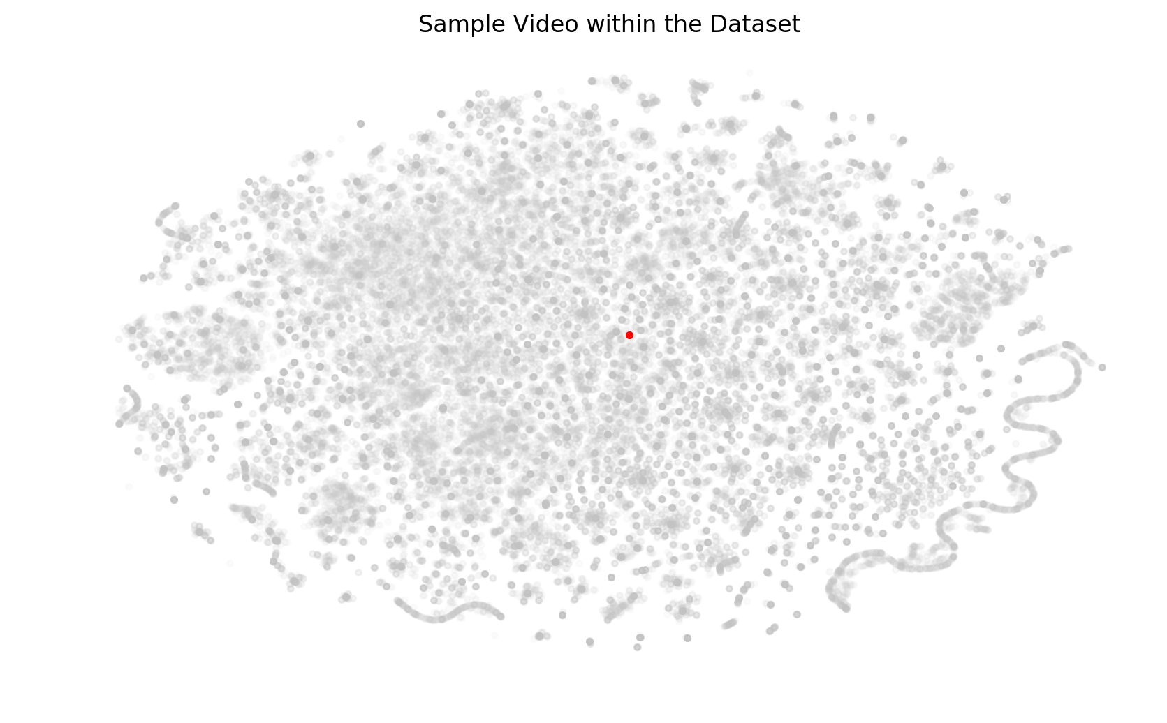
To facilitate plotting the entire dataset, we convert the sampled data into the tSNE representation of the dataset on 2 dimensions. tSNE works by preserving the t-distributions of all the points in the data and projecting these into 2 dimensions so that we can plot it.
s = time()
tX = TSNE(random_state=2020, n_components=2).fit_transform(samplex)
e = time()
print((e-s)/60)
# # save tSNE representation
# with open('../criselle/tsne_cluster_array.pkl', 'wb') as f:
#     pickle.dump(tX, f)
# load tSNE representation
with open('criselle/tsne_cluster_array.pkl', 'rb') as f:
    tX = pickle.load(f)
fig, ax = plt.subplots(dpi=200, figsize=(10,6))
ax.scatter(tX[:,0], tX[:,1], marker='.', c='#BFBFBF', alpha=0.05)
ax.scatter(tX[68587+1,0], tX[68587+1,1], marker='.', color='red')
ax.set_title('Sample Video within the Dataset')
ax.axis('off');
# fig.savefig('sample.png', transparent=True);
5 Results and Discussion
As the method outlined above was created to deal with a situation wherein there will be no more user behavior tracking, the dataset does not include the user-level behaviors and videos. Therefore, in evaluating the results of the recommender system, we can take a look into the different recommended videos of the sample and check which clusters the new recommendations fall under. Instead of validating the recommendations through checking the individual videos of each user, we will be taking a look into the behavior of the recommendations; that is, what how do the recommendations for each cluster actually behave? Do these videos jump from cluster to cluster? Or does this stay within the same relative cluster area?
This behavior of the recommendations can be seen as an indication of the strength of preference of the aggregate users for a given tagset or cluster. The videos whose recommendations tend to not vary, meaning that the videos stay within the same cluster, can be said as having a strong affinity for a given subset of tags and may not be willing to go to different videos.
cluster_counter = []
for key in reco_master.keys():
    user_count = []
    for k, v in reco_master[key]['recos'].items():
        user_count.append(reco_master[key]['recos'][k]['cluster'])
    cluster_counter.append((reco_master[key]['cluster'], user_count))
cluster_counts = df.cluster.value_counts()
for i in range(len(cluster_counter)):
    val = cluster_counter[i]
    cluster_counter[i] = (val[0], val[1], cluster_counts.loc[val[0]])
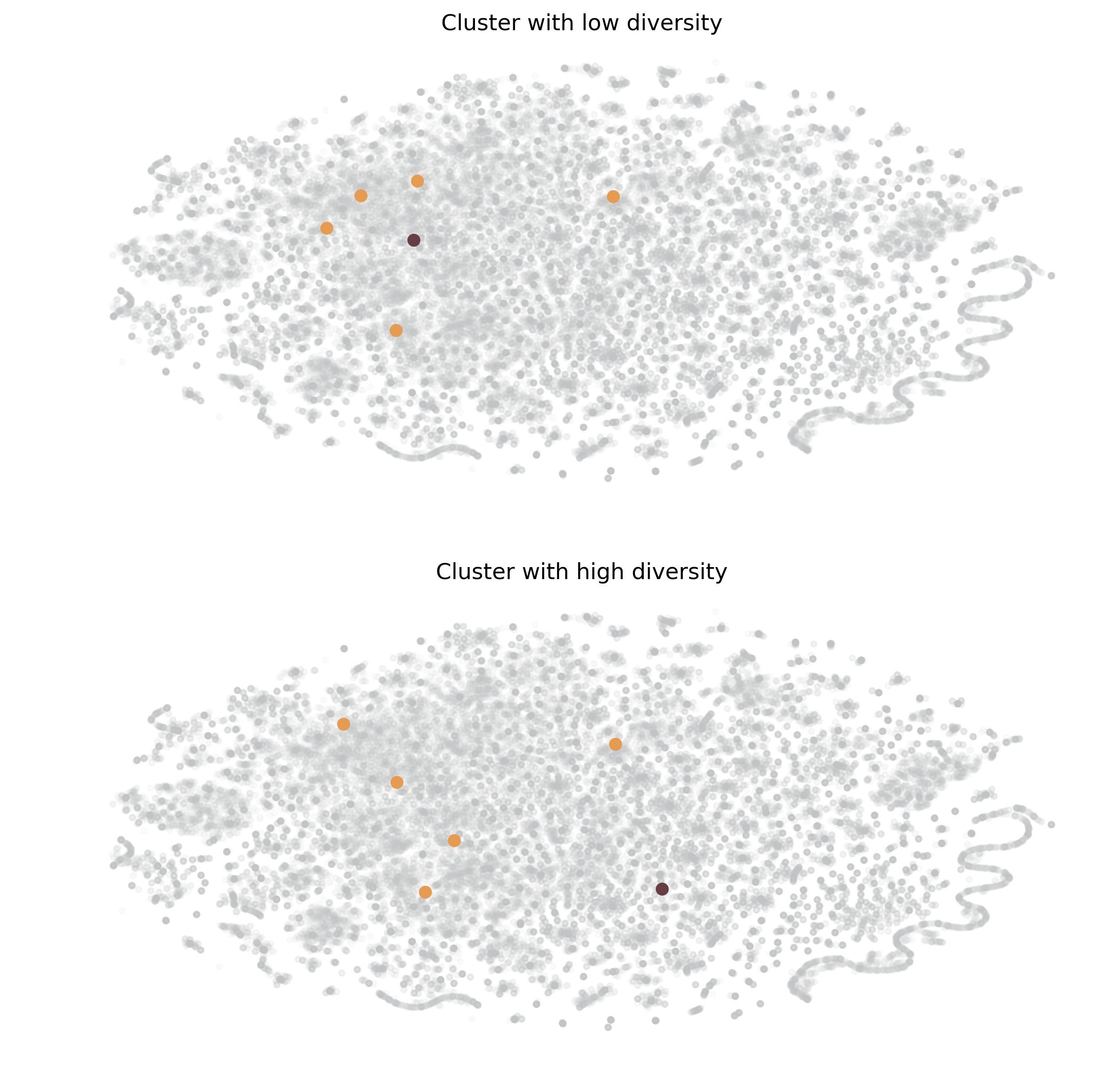
In order to determine how “strong” the persistence or preference of a cluster is in the recommendations, we take a look at the percentage of recommendations per cluster wherein the recommendations are within the same cluster still. That is, how many of the recommendations stay within the same tagsets and how many of these recommendations go to different clusters?
We show this as a percentage of the recommendations that are within the same cluster. In the list below, the lower the percentage is, the more diverse the recommendations, whereas those clusters with a high percentage exhibit a low diversity of recommendations. A low diversity shows that the users who watch these tags in the clusters tend to stick to the same tags when watching.
cluster_counter_res = dict(zip(pd.Series([i[0] for i in cluster_counter]).unique(), [0,]*15))
for i in cluster_counter:
    for reco in i[1]:
        if reco == i[0]:
            cluster_counter_res[i[0]] += 1
        else:
            cluster_counter_res[i[0]] += 0
for k,v in cluster_counter_res.items():
    cluster_counter_res[k] = v/10
print('Diversity of Recommendations (cluster, percentage):')
sorted(tuple(cluster_counter_res.items()), key=lambda x: x[1])
Diversity of Recommendations (cluster, percentage):


[(1, 0.1),
 (10, 0.2),
 (7, 0.4),
 (3, 0.6),
 (13, 0.6),
 (6, 0.7),
 (9, 0.7),
 (12, 0.7),
 (2, 0.8),
 (5, 0.8),
 (4, 0.9),
 (0, 1.0),
 (8, 1.0),
 (11, 1.0),
 (14, 1.0)]
fig, ax = plt.subplots(2,1, dpi=300, figsize=(10,10))
ax[0].scatter(tX[:,0], tX[:,1], color='#BEBFC0', marker='.', alpha=0.05)
ax[0].scatter(tX[reco_master[6086844]['tx_idx'],0], tX[reco_master[6086844]['tx_idx'],1], color='#673E46')
for k,v in reco_master[6086844]['recos'].items():
    ax[0].scatter(tX[v['tx_idx'],0], tX[v['tx_idx'],1], color='#E59B51')
ax[0].axis('off')
ax[0].set_title('Cluster with low diversity')
ax[1].scatter(tX[:,0], tX[:,1], color='#BEBFC0', marker='.', alpha=0.05)
ax[1].scatter(tX[reco_master[288740]['tx_idx'],0], tX[reco_master[288740]['tx_idx'],1], color='#673E46')
for k,v in reco_master[288740]['recos'].items():
    ax[1].scatter(tX[v['tx_idx'],0], tX[v['tx_idx'],1], color='#E59B51')
ax[1].axis('off')
ax[1].set_title('Cluster with high diversity');
6 Conclusion
This study shows one potential implementation of a recommender system given the hypothetical scenario wherein companies and websites will not be allowed to track user behavior in their sites. The recommender system shows that there are other approaches that may be explored in determining new recommendations for users. Using the Pornhub database, we were able to create a recommender system that uses a two-fold method, association rules and unsupervised clustering, to arrive at potential recommendations for a given user watching a given video.
Some advantages of this approach are that:
- There is no need to track individual users. The aggregate of all users is used instead as a group behavior and the association rules and unsupervised clustering are performed on this aggregated set.
- This approach limits the cold-start problem typically faced by some recommender systems. This is inherently due to the non-collection of user-specific data. Whereas tradtional systems like user-based collaborative filtering or alternating least squares rely on building up a database for each user’s activity, the approach presented here only necessitates that the user interact at least once with the system for us to generate recommendations.
However, there are some disadvantages:
- Accuracy will most likely be lower than traditional user-specific recommender systems. This is due to the fact that the recommendations generated using this approach is more attuned to a stereotype of a user, rather than just a specific user. User-based collaborative filtering methods and alternating least squares, on the other hand, use actual user-level data that could lead to higher accuracy and more optimization. This also allows for better individual targeting of users. However, the tradeoff is that users will have to be willing to give up their personal data.
In further pursuing this method, one can look into obtaining a user-specific or user-level data for the same dataset with the aim of comparing the results of a traditional recommender system against our method. We were unable to get the user-level data due to privacy concerns and it would be beneficial to benchmark the performance of the system presented here against a user-level approach. Additionally, the user-level data can provide more insights on the recommendations created by the approach detailed here, as well as present more opportunities to fine-tune the recommendations against the “truth” data.
The method outlined here has shown some promise at the task of generating recommendations when there is not universe of user-level interactions that could be accessed. This method has some room for improvements that could be gained by comparing against the truth-level data of per-user.
7 Acknowledgements
We would like to thank the MSDS Professors Dr Christopher Monterola, Dr Erika Legara, and of course our BDCC professor, Dr Christian Alis for imparting the necessary skills and knowledge necessary to finish this project. We would also like to thank ACceSS lab scientists, ASITE admin and staff, and our MSDS 2020 classmates for the never ending support. Special mention to Jeff Go for pointing us to the correct download link for the dataset.
8 References
[1] K. Feher, “Digital identity and the online self: Footprint strategies – An exploratory and comparative research study,” J. Inf. Sci., 2019.
[2] J. Isaak and M. J. Hanna, “User Data Privacy: Facebook, Cambridge Analytica, and Privacy Protection,” Computer (Long. Beach. Calif)., 2018.
[3] B. Zhang, N. Wang, and H. Jin, “Privacy Concerns in Online Recommender Systems: Influences of Control and User Data Input,” SOUPS ’14 Proc. Tenth Symp. Usable Priv. Secur., 2014.
[4] M. Fleischman and E. Hovy, “Recommendations without user preferences: A natural language processing approach,” in International Conference on Intelligent User Interfaces, Proceedings IUI, 2003.
9 APPENDIX
9.1. <a href=preprocessing.ipynb>Preprocessing</a>
9.2. <a href=EDA.ipynb>EDA</a>
9.3. Association Rule Mining
9.4. Clustering
Pickle files not attached to submission due to size. Files can be accessed here: s3://bdcc-cdavid