
Topic Modelling of Subreddit Clusters
Published:
Overview
This technical report was a requirement for my Data Mining and Wrangling Lab held under Professor Erika Legara as part of MSc in Data Science. In this technical report, we were tasked with using identifying the potential subreddits by using unsupervised machine learning techniques. I apply word vectorization, principal component analysis, KMeans Clustering, and Non-Negative Matrix Factorization methods to determine the optimal number of original subreddits.
import numpy as np
import pandas as pd
import matplotlib.pyplot as plt
%matplotlib inline

from sklearn.datasets import load_wine, fetch_20newsgroups
from sklearn.preprocessing import StandardScaler
from sklearn.feature_extraction.text import TfidfVectorizer
from sklearn.manifold import TSNE
from sklearn.decomposition import TruncatedSVD
from scipy.spatial.distance import euclidean, cityblock

from IPython.display import HTML
import re
import seaborn as sns
from collections import Counter
import string

from sklearn.cluster import KMeans
from scipy.cluster.hierarchy import linkage, dendrogram
from sklearn.feature_extraction.text import CountVectorizer
Executive Summary
Reddit is a social news aggregation and discussion board website that was ranked as the number 21 most visited site in the world in 2019. Users are able to upload images, links, text, and other file formats into different sub-topic discussion boards called subreddits. These subreddits encompass a wide range of topics, with the top subreddits being r/funny, r/AskReddit, r/todayilearned, r/worldnews, and r/Science. The objective of this analysis is to determine whether there are topic clusters that would form based on a sample of 6,000 topics or posts from various subreddits. Given that each specific subreddit would be dedicated to its own topic, this analysis proposes to use unsupervised clustering to determine whether the sample of 6,000 posts would cluster together by their original topic/subreddit.
Using hierarchical clustering with Ward’s method, the optimal number of clusters was deemed to be 6. These 6 distinct topics are: democratic party, republican party, new year resolution, technical support, new years, til (today I learned). Among these clusters, the “til” cluster dominates and contains most of the documents; this could be due to the generalized nature of the topics inside the subreddit r/todayilearned which causes it to be lumped together with different topics. Further analysis may still be done using different clustering methods.
Data Description
The data that will be analyzed is a csv file containing a sample of 6,000 posts from different subreddits collected from reddit.com. These posts include only the topic header or title and username or author of the post and do not include other details such as date, time, comments, and others.
df = pd.read_csv('reddit-dmw-sample.txt', sep='\t', usecols=['author', 'title'])
df.head(2)
| author | title | |
|---|---|---|
| 0 | PrimotechInc | 7 Interesting Hidden Features of apple ios9 |
| 1 | xvagabondx | Need an advice on gaming laptop |
Workflow
In analyzing the data, the following workflow will be used to explore, clean, and prepare the data for modelling/clustering:
- Data Processing
- remove punctuations in preparation for vectorization
- convert all letters to lowercase
- remove duplicate entries
- lemmatize similar words
- Exploratory Data Analysis (EDA)
- analyze distribution of authors/titles
- check for frequency of words
- check for duplication of entries
- Modelling
- vectorize into bag of words (bow)
- run clustering algorithm
- validate optimal number of
kclusters - extrapolate topics/themes from each cluster
- Conclusion/Summary
Data Processing
To process this data, we first clean up the title text by converting all into lowercase. Additionally, all punctuations are removed and only characters that are alphanumeric or spaces are retained. After this preprocessing, all duplicated text in title_clean are dropped, keeping only those first instances of the text. This is to ensure that the clustering will not be skewed by multiple entries of the same title. There are also columns title_len and title_words created which contain the character length of the title and the number of words in the title respectively. This is done for EDA purposes later on. In total, the following things have been done to clean up the data:
- convert titles to lowercase
- remove all punctuations
- drop all duplicated titles
- create new columns
title_lenandtitle_wordsfor EDA
df['title_lower'] = df['title'].apply(lambda row: row.lower())
df['title_clean'] = df['title_lower'].apply(lambda row: re.sub(r'[^\w\s]', '', row))
df.drop_duplicates(subset='title_clean', keep='first', inplace=True)
df.reset_index(inplace=True, drop=True)
df['title_len'] = df['title_clean'].apply(lambda row: len(row))
df['title_words'] = df['title_clean'].apply(lambda row: len(row.split()))
One of the potential problems that we may encounter in clustering the titles and extracting themes is the breadth of the english language. In normal speech, people use different words to express the same ideas, thoughts, or feelings. There are also pluralizations of words that will render each word as different from its plural form. In order to condense the information into their base meaning, a process called Lemmatization is applied to the cleaned titles. Lemmatization works by converting different forms of the same word into a single word, thus condensing these words back into their root or base meaning. This process is not 100% accurate however, but for the purposes of this analysis, the Lemmatization process is deemed to be beneficial in order to generate a more accurate result.
The following Lemmatization will be conducted on title_clean for the following word types:
- verbs
- adjectives
- adverbs
Nouns will be excluded from the Lemmatization as the lemmatization of nouns may have a high rate of error given the different names that may appear in the data.
from nltk.stem import WordNetLemmatizer

lemmatizer = WordNetLemmatizer()

lemm_verb = [' '.join([lemmatizer.lemmatize(word, pos='v') for word in
                 text.lower().replace("\n", " ").split(" ") if len(word) > 1])
       for text in df['title_clean']]
lemm_adj = [' '.join([lemmatizer.lemmatize(word, pos='a') for word in text.split(" ")
                 if len(word) > 1]) for text in lemm_verb]
lemm_ad = [' '.join([lemmatizer.lemmatize(word, pos='r') for word in text.split(" ")
                 if len(word) > 1]) for text in lemm_adj]

# create new column in dataframe
df['title_lem'] = lemm_ad
Exploratory Data Analysis
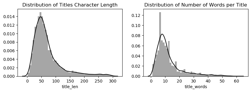
In the initial data exploration, we look into the basic features of our dataset. This includes the distribution of titles, authors, posts, character lengths, and others. The information extracted may give a better picture of the dataset.
fig, ax = plt.subplots(1, 2, dpi=100, figsize=(10,3))
sns.distplot(df['title_len'], kde=True, kde_kws={'color':'k'},
             hist_kws={'color':'grey', 'alpha':0.7}, ax=ax[0])
ax[0].set_title('Distribution of Titles Character Length')
sns.distplot(df['title_words'], kde=True, kde_kws={'color':'k'},
            hist_kws={'color':'grey', 'alpha':0.7}, ax=ax[1])
plt.title('Distribution of Number of Words per Title')
print(f'Mean Title Words: {df.title_words.mean()}')
print(f'Mean Title Character Length: {round(df.title_len.mean(), 2)}');
Mean Title Words: 12.166266300617707
Mean Title Character Length: 70.29
Aside from the distribution of the title lengths and character lengths, since the dataset consists of posts from subreddits and these are user-generated meaning that these follow human speech patterns, we assume that this would follow Zipf’s Law. This would determine that the frequency of the top 20 words would account for 80% of the total frequency of words and thus would manifest in a power law when plotted on a log-log scale. The dataset used here would be the Lemmatized titles with stop words being removed. In order to achieve this, we use CountVectorizer package to automatically get the counts of each word and remove the english stop words; we then pass this into a dataframe and collect the data from there.
cv = CountVectorizer(token_pattern=r'[a-z-]+', stop_words='english')
tf = cv.fit_transform(df['title_lem'])
tf_feature_names = cv.get_feature_names()
df_cv = pd.DataFrame(tf.toarray(), columns=tf_feature_names)
lem_words = list(df_cv.columns)
lem_vals = [df_cv[i].sum() for i  in lem_words]
top_words_lem = list(zip(lem_words, lem_vals))
top_words_lem.sort(key=(lambda x: x[1]), reverse=True)
fig, ax = plt.subplots(1, 2, dpi=100, figsize=(10,3))
sns.lineplot([i for i in range(len(top_words_lem[:1000]))],
             [i[1] for i in top_words_lem[:1000]], ax=ax[0])
ax[0].set_title('Top Words by Frequency')
ax[0].set_ylabel('Frequency')
ax[0].set_xlabel('Word Rank')
sns.lineplot(np.log([i for i in range(1, len(top_words_lem[:1001]))]),
             np.log([i[1] for i in top_words_lem[:1000]]), ax=ax[1])
ax[1].set_title('Top Words by Frequency (Log-Log Scale)')
ax[1].set_ylabel('(Log) Frequency')
ax[1].set_xlabel('(Log) Word Rank');
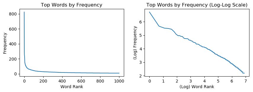
As suspected, the distribution of the top 1,000 words follows a power law curve when plotted on the log-log scale and gives us an idea of the frequency of the themes. Subreddits typically follow a post pattern wherein each post would follow a specific format, i.e. for the subreddit todayilearned, each post typically starts with TIL followed by the text. Combined with the knowledge that the word distribution follows a power law curve, we may assume that the top 100 or 200 words in the titles would account for the themes of the posts.
To better visualize the top words before clustering, we create a wordcloud of the top terms of the lemmatized titles:
# Check the common words in the lemmatized titles
from wordcloud import WordCloud, STOPWORDS
text = df['title_lem']
wordcloud = WordCloud(scale=3,
    background_color = 'white',
    stopwords = STOPWORDS).generate(str(text))
fig = plt.figure(
    edgecolor = 'k',
    dpi=300)
plt.imshow(wordcloud, interpolation='bilinear', cmap='Blues')
plt.axis('off')
plt.tight_layout(pad=0)
plt.show()
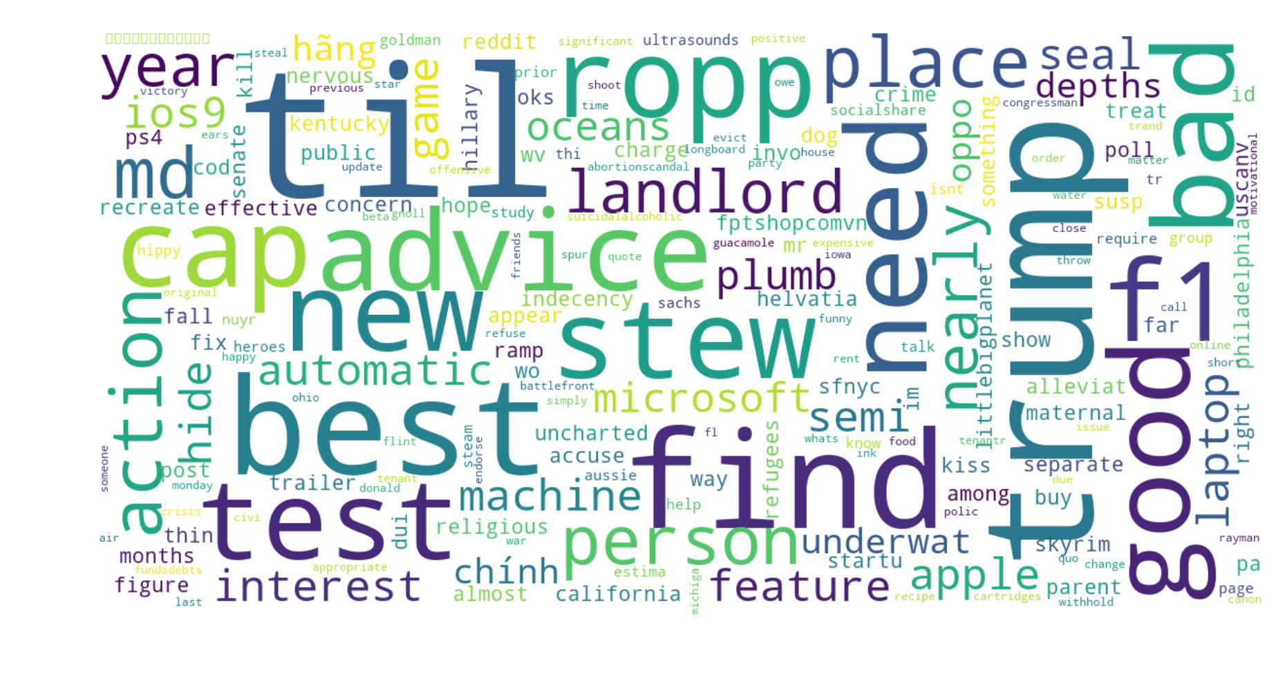
Based on this word cloud, some of the top terms are “til” and “trump”. “til” is the specific pattern used for topic headers for reddit.com/r/todayilearned subreddit, as such we can expect that there should be a cluster of subreddit topics coming from this subreddit. As “trump” is also in the top terms, we expect that there would be a politically-relevant cluster of themes perhaps focused on the 2016 presidential campaign, United States President, Republican party, or other similar topics.
Model
Vectorize into Bag of Words
In the intial stage of clustering, we vectorize all the words in titles into a bag-of-words representation. Essentially, this converts all the words in all the titles into columns of a dataframe, where the occurence/frequency of each word is mapped per row or title. There are two main methods to conduct this vectorization:
- CountVectorizer
- Creates a matrix of word counts
- Counts are not normalized
- Term Frequency Inverse Document Frequency (TF-IDF) Vectorizer
- Term Frequency is essentiall the same as CountVectorizer
- Inverse Document Frequency assigns a weight to the count by dividing the term frequency count by the total number of times the term appears in other documents
For this analysis, we will be using TF-IDF as this accounts for the weights of the frequencies of the words that appear in other documents. This would give us a better representation of the “weight” of the specific term with regard to all the other documents in the titles. In running the TFIDF Vectorizer, we place the following parameters:
- token_pattern =
r[a-z-]+- this regular expression returns only words that match and ensures that we are left with letters and filters out all numeric characters - stop_words =
english- this parameter ensures that we filter out all english stop words such as “the”, “as”, “is”, etc. as these are deemed not to contain any relevant information in topic extraction for our purposes. - min_df =
0.000167- this represents 1/6000 occurences in the corpus. The parameter filters out those words that only occur once in all the titles as these words are one-offs and are deemed not relevant to the topic extraction. - ngram_range =
(1, 2)- this parameter allows the tfidf vectorizer to analyze word combinations of up to 2 words in length. As the subreddit topics are written in natural/human language, there are words strung together such as first and last names, places, and other two-word terms that will not be accounted for if we were to vectorize word-by-word only. The ngrams_range parameter ensures that we are able to extract and vectorize combinations of 2 words to see whether these drive the themes in the corpus.
# TFIDF Vectorizer and Bag of Words
tfidf_vectorizer = TfidfVectorizer(token_pattern=r'[a-z-]+',
                                   stop_words='english', min_df=0.000167,
                                  ngram_range=(1,2))
bows = tfidf_vectorizer.fit_transform(df['title_lem'])
tfidf_features = tfidf_vectorizer.get_feature_names()
df_tfidf = pd.DataFrame(bows.toarray(), columns=tfidf_features)

# Count Vectorizer and term frequency (tf)
cv = CountVectorizer(token_pattern=r'[a-z-]+', min_df=1, stop_words='english')
tf = cv.fit_transform(df['title_lem'])
tf_feature_names = cv.get_feature_names()
Dimensionality Reduction (LSA)
To expediate the analysis of the data, we perform dimensionality reduction on the features. Dimensionality reduction involves selecting the top eigenvectors of the bag-of-words matrix in order to reduce the number of total features or words that need to be processed. This often necessitates the use of Principal Component Analysis (PCA) to determine the eigenvectors that have the highest determination with regard to the total explained variance of the matrix. In this analysis, the method to be used in dimensionality reduction would be Latent Semantic Analysis (LSA), the sklearn implementation of which is TruncatedSVD. LSA differs from PCA in that the points are not mean-centered prior to dimensionality reduction, and works on a term frequency matrix constructed from documents. As such, LSA is most often used on document and bag-of-words and not PCA.
In order to account for the total explained variance we want to predict, we first run an iterative method to compute for the total explained variance for different n_components to be used for our TruncatedSVD/LSA:
# check for the components and their explained variance
components_list = [i for i in range(500,1501,200)]
var_ex = []
for n in components_list:
    tsvd_iter = TruncatedSVD(n_components=n, random_state=1337)
    tsvd_iter.fit_transform(bows)
    print(f'Components: {n}, explained variance: {tsvd_iter.explained_variance_.sum() * 100}.')
    var_ex.append(tsvd_iter.explained_variance_.sum() * 100)
plt.plot(components_list, var_ex)
plt.title('Explained Variance per No. of Components')
plt.ylabel('Explained Variance (%)')
plt.xlabel('Number of Components');
Components: 500, explained variance: 24.150074740050037.
Components: 700, explained variance: 29.805413177170504.
Components: 900, explained variance: 34.73927974627129.
Components: 1100, explained variance: 39.16318067420884.
Components: 1300, explained variance: 43.2078809840597.
Components: 1500, explained variance: 46.97871182774863.
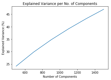
As we’ve seen in the EDA, natural human language follows a Zipf’s Law or a power law curve. As such, we assume that the top occurring words in the document, without stop words, would be most predictive in terms of the topic or theme that the title belongs to. We deem that an explained variance of around 25% would be sufficient in our analysis to be able to determine the topic/theme for clustering.
# Truncated SVD and TSNE variables
TSVD = TruncatedSVD(n_components=500, random_state=1337)
X_bow = TSVD.fit_transform(bows)
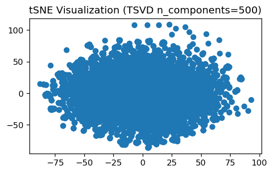
X_bow_new = TSNE(n_components=2, random_state=1337).fit_transform(X_bow)
Since we are left with 500 components, we use the t-distributed Stochastic Neighbor Embedding (tSNE) algorithm to be able to reduce these to 2 dimensions for visualization purposes. tSNE works by using a t-distribution to determine the relationship of points in higher dimension space. This is then projected on to 2 dimensions (or more, to be determined with the n_components parameter) as random points and the t-distribution is used to incrementally move each point to fit into its originally computed t-distribution and end up with a 2-dimensional representation of the higher dimensional points. Due to this, tSNE is helpful in visualizing the clusters but does not preserve the exact relationship between points.
# plot TSNE visualization
Clustering
In unsupervised clutering, there are generally two approaches used: representative based or agglomerative/hierarchical clustering. KMeans clustering is most commonly used for representative based clustering, however, this method would necessitate a guess on the initial number of clusters and will cluster based on this guess. Therefore, for the analysis of natural language such as subreddit topics, this approach may not result in the cleanest results.
For Hierarchical clustering on the other hand, we can use agglomerative hierarchical clustering. This method initially treats each individual point as a singleton and clusters based on the closest points near to this until a certain metric is reach, which would determine the number of optimal clusters. The benefit of using this approach is that each individual point, and in the case of this analysis, individual word, will be considered its own singleton at the beginning and will be clustered with its nearest points. The downside of using this approach is that it requires higher computational power as the algorithm will need to parse every data point and cluster from the bottom-up.
For the purposes of this analysis, we will be using agglomerative hierarchical clustering using Ward’s method. This method uses the distance between two clusters, taken as the sum of squares between two points, and uses the amount that this sum of squares will increase when we merge two points as the main “stopping” point for clustering. This method has the benefit of measuring the “cost” of merging two clusters as it tries to merge the most number of points while minimizing the change/increase in the sum of squares between the merged points.
from scipy.cluster.hierarchy import linkage, dendrogram
Z = linkage(X_bow, method='ward', optimal_ordering=True)
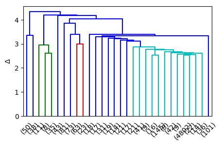
To visualize the clustering, we will use a dendrogram which shows the links between the clusters with a different color “stem” per cluster.
fig, ax = plt.subplots(figsize=(5,3), dpi=100)
dn = dendrogram(Z, ax=ax, truncate_mode='lastp')
ax.set_ylabel(r'$\Delta$');
In order to determine the optimal number of clusters, we use the Elbow Method which computes the largest differences in the sum of squares distance between different values of k. The maximum drop is used as the optimal number of k clusters.
fig, ax = plt.subplots(figsize=(6,4), dpi=120)

last = Z[-10:, 2]
last_rev = last[::-1]
idxs = np.arange(1, len(last) + 1)
ax.plot(idxs, last_rev, label='Distance')

acceleration = np.diff(last, 2)
acceleration_rev = acceleration[::-1]
ax.plot(idxs[:-2] + 1, acceleration_rev, label='Drop in Distance')
k = acceleration_rev.argmax() + 2
ax.set_title('Elbow Method Validation for Hierarchical Clustering')
ax.set_ylabel('Distance')
ax.set_xlabel('Number of Clusters')
print('Ideal number of clusters:', k)
ax.legend();
Ideal number of clusters: 6
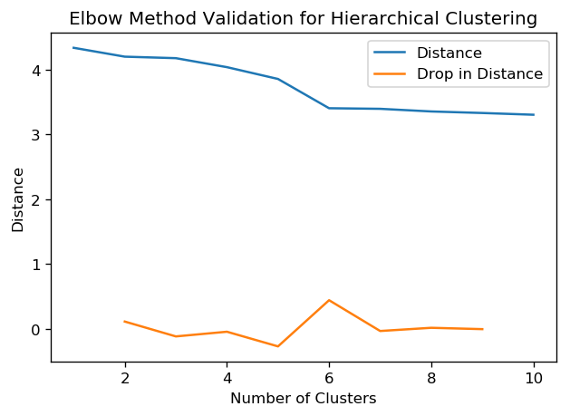
From the result of the Elbow Test, the optimal number of clusters is 6. We visualize this by using the scipy library called fcluster which takes the cluster from our linkage created previously and extrapolates the clustering based on a user-determined number of clusters in the parameter t.
from scipy.cluster.hierarchy import fcluster

y = fcluster(Z, t=k, criterion='maxclust')

fig, ax = plt.subplots(1, 2, dpi=120, figsize=(10,3))
ax[0].scatter(X_bow_new[:,0], X_bow_new[:,1], c=y, alpha=0.3)
ax[1].bar(Counter(y).keys(), Counter(y).values())
ax[1].set_title('Number of Documents per Cluster')
ax[1].set_xlabel('Cluster Number')
ax[1].set_ylabel('Number of Documents')
print(Counter(y));
Counter({6: 5403, 5: 159, 1: 88, 4: 81, 2: 54, 3: 43})
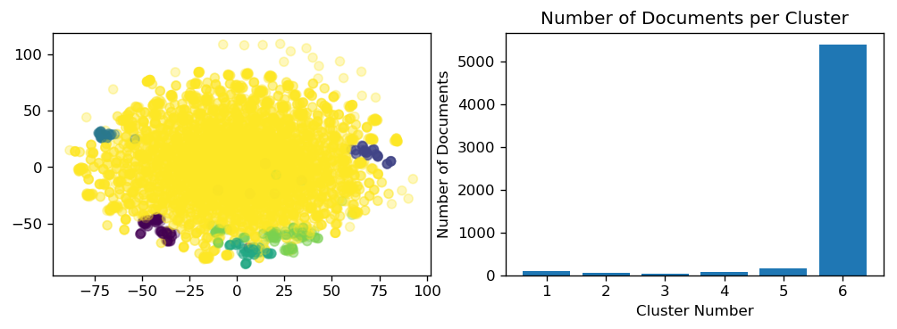
The clustering using hierarchical clustering with Wards method seems to prefer clustering all the topics into one cluster only. This could be the result of having a lot of the topics be very diverse and thus the clustering cannot detect a definitive cluster for this group of topics. Below we take a look at the top topics or terms for each cluster to perform a sanity check on the clusters.
from scipy.cluster.hierarchy import fcluster

df_tfidf['cluster'] = pd.Series(y)
clusters = pd.DataFrame()
for i in range(1, 7):
    clusters['cluster ' + str(i)] = df_tfidf[df_tfidf['cluster'] == i].sum(
        axis=0)[:-1].nlargest(100).index
clusters.head(15)
| cluster 1 | cluster 2 | cluster 3 | cluster 4 | cluster 5 | cluster 6 | |
|---|---|---|---|---|---|---|
| 0 | new | number | n | trump | sanders | til |
| 1 | new year | support | t | donald | bernie | game |
| 2 | new years | technical | m | donald trump | bernie sanders | make |
| 3 | year | phone number | c | rally | clinton | new |
| 4 | years | technical support | ng | til donald | hillary clinton | trump |
| 5 | happy new | phone | ch | trump rally | hillary | use |
| 6 | happy | hotmail | l | endorse | need | |
| 7 | years eve | tech support | b | john oliver | super | just |
| 8 | eve | support phone | ngon | oliver | super tuesday | time |
| 9 | years day | toll | h | john | tuesday | best |
| 10 | day | toll free | l m | students | clinton email | help |
| 11 | surf | tech | u | endorse donald | state | food |
| 12 | turf | support number | s | til | iowa | car |
| 13 | years resolution | dial | m n | black students | vote | sanders |
| 14 | game | tollfree | th | remove | soros | question |
Based on the results of the hierarchical clustering, there are 6 distinct clusters in the sample text:
- Cluster 1: This cluster is mostly regarding new years and new years resolutions.
- Cluster 2: This cluster is mostly about techinical support and probably gadget support or help
- Cluster 3: This cluster is composed on non-sensical words. The reason for this is probably due to the foreign words (Vietnamese, Russian, etc.) in the original sample text.
- Cluster 4: This cluser is mostly concerned with donald trump, and rallies. One can assume that this cluster is mostly representative of either the Presidential Republican campaign of 2016.
- Cluster 5: This cluster is the opposite of Cluster 4, this regards more of Bernie Sanders and Hillary Clinton or more of the Democratic campaign.
- Cluster 6: The biggest cluster, this cluster contains a lot of the TIL (todayilearned) topics, mixed in with other topics.
Conclusion and Results
Using hierarchical clustering with Ward’s method, we were able to determine an optimal number of 6 clusters for the sample set of 6,000 topics from different subreddits. For the most part, these clusters contained specific topics that were related to each other, however, looking at the distribution of documents per cluster, it seems that once cluster dominates all the others in terms of the number of documents. This could be due to the subjective nature of the unsupervised clustering that was implemented, as the topics or terms in the documents pertaining to cluster number 6 could be too mixed or general that the unsupervised clustering was not able to separate them into distinct clusters. Overall, results of the clustering show 5 distinct topics and one cluster that is a mix of all the documents that may not have been distinguished by the algorithm.
Different or more advanced clustering methods may be used to further tweak the clustering performed. These include the use of NMF (Non-negative Matrix Factorization) or LDA (Latent Dirichlet Allocation), which utilizes a different algorithm to determine clusters.
Addendum: Non-Negative Matrix Factorization
As mentioned above, there can be further clustering methods explored to cluster the dataset. This includes the use of Non-negative Matrix Factorization or (NMF). NMF is a version of matrix decomposition that operates on the transposed bag of words matrix and decomposes a matrix A into VH such that A = VH.
In order to determine the optimal number of k for the NMF, we use a coherence score that uses the word2vec library of sklearn. This code below is edited from: Derek Greene’s code which can be found at https://github.com/derekgreene/topic-model-tutorial/blob/master/3%20-%20Parameter%20Selection%20for%20NMF.ipynb
tfidf_vectorizer = TfidfVectorizer(token_pattern=r'[a-z-]+',
                                   stop_words='english', min_df=3)
bows = tfidf_vectorizer.fit_transform(df['title_lem'])
terms = tfidf_vectorizer.get_feature_names()
A = bows
kmin = 4
kmax = 10
from sklearn import decomposition
topic_models = []
# try each value of k
for k in range(kmin,kmax+1):
    print("Applying NMF for k=%d ..." % k)
    # run NMF
    model = decomposition.NMF(init="nndsvd", n_components=k)
    W = model.fit_transform(A)
    H = model.components_
    # store for later
    topic_models.append((k,W,H))
Applying NMF for k=4 ...
Applying NMF for k=5 ...
Applying NMF for k=6 ...
Applying NMF for k=7 ...
Applying NMF for k=8 ...
Applying NMF for k=9 ...
Applying NMF for k=10 ...
import re
class TokenGenerator:
    def __init__(self, documents, stopwords):
        self.documents = documents
        self.stopwords = stopwords
        self.tokenizer = re.compile( r"[a-z-]+" )

    def __iter__(self):
        print("Building Word2Vec model ...")
        for doc in self.documents:
            tokens = []
            for tok in self.tokenizer.findall(doc):
                if tok in self.stopwords:
                    tokens.append("<stopword>")
                elif len(tok) > 0:
                    tokens.append(tok)
            yield tokens
raw_documents = []
for i in df['title_lem']:
    raw_documents.append(i)
custom_stop_words = []
import gensim
docgen = TokenGenerator(raw_documents, custom_stop_words)
# the model has 500 dimensions, the minimum document-term frequency is 20
w2v_model = gensim.models.Word2Vec(docgen, size=500, min_count=3, sg=1)
Building Word2Vec model ...
Building Word2Vec model ...
Building Word2Vec model ...
Building Word2Vec model ...
Building Word2Vec model ...
Building Word2Vec model ...
print("Model has %d terms" % len(w2v_model.wv.vocab))
Model has 3248 terms
def calculate_coherence(w2v_model, term_rankings):
    overall_coherence = 0.0
    for topic_index in range(len(term_rankings)):
        # check each pair of terms
        pair_scores = []
        for pair in combinations(term_rankings[topic_index], 2):
            pair_scores.append(w2v_model.similarity(pair[0], pair[1]))
        # get the mean for all pairs in this topic
        topic_score = sum(pair_scores) / len(pair_scores)
        overall_coherence += topic_score
    # get the mean score across all topics
    return overall_coherence / len(term_rankings)

def get_descriptor(all_terms, H, topic_index, top):
    # reverse sort the values to sort the indices
    top_indices = np.argsort(H[topic_index,:])[::-1]
    # now get the terms corresponding to the top-ranked indices
    top_terms = []
    for term_index in top_indices[0:top]:
        top_terms.append(all_terms[term_index])
    return top_terms
k_values = []
coherences = []
terms = tfidf_vectorizer.get_feature_names()
for (k,W,H) in topic_models:
    # Get all of the topic descriptors - the term_rankings, based on top 10 terms
    term_rankings = []
    for topic_index in range(k):
        term_rankings.append(get_descriptor(terms, H, topic_index, 10))
    # Now calculate the coherence based on our Word2vec model
    k_values.append(k)
    coherences.append(calculate_coherence(w2v_model, term_rankings))
    print("K=%02d: Coherence=%.4f" % (k, coherences[-1]))
K=04: Coherence=0.9730
K=05: Coherence=0.9733
K=06: Coherence=0.9747
K=07: Coherence=0.9769
K=08: Coherence=0.9778
K=09: Coherence=0.9762
K=10: Coherence=0.9792


/anaconda3/lib/python3.7/site-packages/ipykernel_launcher.py:7: DeprecationWarning: Call to deprecated `similarity` (Method will be removed in 4.0.0, use self.wv.similarity() instead).
  import sys
fig = plt.figure(figsize=(13,7))
# create the line plot
ax = plt.plot( k_values, coherences )
plt.xticks(k_values)
plt.xlabel("Number of Topics")
plt.ylabel("Mean Coherence")
# add the points
plt.scatter( k_values, coherences, s=120)
# find and annotate the maximum point on the plot
ymax = max(coherences)
xpos = coherences.index(ymax)
best_k = k_values[xpos]
plt.annotate( "k=%d" % best_k, xy=(best_k, ymax), xytext=(best_k, ymax), textcoords="offset points", fontsize=16)
# show the plot
plt.show()
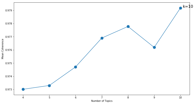
Based on the cohesion score above, the optimal number of k clusters is 10. Running the NMF model below with 10 clusters, we get the topics:
from sklearn.decomposition import NMF, LatentDirichletAllocation
from sklearn.preprocessing import normalize

clusters = 10

# Run NMF
nmf = NMF(n_components=clusters, random_state=1337, alpha=.1,
          l1_ratio=.5, init='nndsvd')
nmf_trans = nmf.fit_transform(normalize(bows))
def display_topics(model, feature_names, no_top_words):
    for topic_idx, topic in enumerate(model.components_):
        print("Topic %d:" % (topic_idx + 1))
        print( ", ".join([feature_names[i]
                        for i in topic.argsort()[:-no_top_words - 1:-1]]))

no_top_words = 15
print('Clustering with NMF')
display_topics(nmf, tfidf_vectorizer.get_feature_names(), no_top_words)
Clustering with NMF
Topic 1:
game, play, video, like, pc, best, steam, year, abcya, compare, anticipate, time, release, nintendo, montage
Topic 2:
til, use, people, world, state, know, years, unite, kill, thing, actually, million, water, old, man
Topic 3:
sanders, bernie, iowa, campaign, vote, win, supporters, candidate, raise, voters, tuesday, lead, poll, say, presidential
Topic 4:
new, year, happy, years, day, eve, york, start, resolution, time, old, birthday, apple, hampshire, amaze
Topic 5:
trump, donald, rally, iowa, endorse, rubio, oliver, poll, supporters, disgust, cruz, john, white, say, tuesday
Topic 6:
make, good, pizza, easy, perfect, dinner, tomorrow, english, home, foods, today, time, use, sure, cake
Topic 7:
need, help, advice, legal, life, friend, pay, probably, laptop, speed, agreement, issue, understand, read, situation
Topic 8:
clinton, hillary, email, iowa, caucus, state, release, poll, say, obama, clintons, president, super, democratic, soros
Topic 9:
n, m, t, c, ng, l, s, ch, b, u, th, ngon, d, h, o
Topic 10:
support, number, technical, phone, tech, hotmail, free, toll, dial, tollfree, antivirus, dell, line, kindle, norton
It seems that overall, the NMF clustering worked better than the original hierarchical clustering with Ward’smethod. Specifically, this was able to parse more topics (10) than the hierarchical clustering. The topics include:
- Topic 1: video games
- Topic 2: todayilearned(TIL)
- Topic 3: Bernie Sanders, votes
- Topic 4: new year
- Topic 5: Donald Trump, rally
- Topic 6: food
- Topic 7: help/advice
- Topic 8: Hillary Clinton, email, caucus
- Topic 9: foreign words, single letters
- Topic 10: Technical support
With more tweaking and adjustments to the tokenization and word2vec implementation, the NMF approach may still yield better results.
Acknowledgements:
I would like to thank the following people for their invaluable contributions to the creation of this analysis:
- My LT (redacted for anonymity)
- MSDS 2020: Raph Ongleo, Ella Manasan, Criselle David, Lance Sy, Nigel Silva, Benj Danao
- MSDS 2019: Patricia Manasan
- Paper: Subtopics in News Articles about Artificial Intelligence in the Last 30 Days by Anthony Dy and Marlon Teodosio
- Dimensionality Reduction Notebook by Christian Alis
- Ed David
- https://www.geeksforgeeks.org/python-lemmatization-with-nltk/
- https://blog.acolyer.org/2019/02/18/the-why-and-how-of-nonnegative-matrix-factorization/
- https://medium.com/nanonets/topic-modeling-with-lsa-psla-lda-and-lda2vec-555ff65b0b05
- https://github.com/derekgreene/topic-model-tutorial/blob/master/3%20-%20Parameter%20Selection%20for%20NMF.ipynb
- https://medium.com/mlreview/topic-modeling-with-scikit-learn-e80d33668730