
Unsupervised Clustering Analysis of NBA Players
Published:
Overview
This technical report was created for our Data Mining and Wrangling class in AIM MSDS. In particular, this was done during our 2nd semester of class, as one of the required lab reports. In this report, we sought to understand how the landscape of the NBA has changed over the decades, and specifically if we are able to generalize certain player stereotypes throughout the years. We analyze these stereotypes, as well as the changes among them, using Unsupervised Clustering and apply Principal Component Analysis to extract meaningful features from the data. At the end, we also take a look at the evolution of 3-point shooters and the dramatic change that the 3-point shot has introduced to the NBA gameplay (as part of my personal interest, mostly).
Acknowledgements
This analysis was done together with my Lab partner, Lance Aven Sy.
Imports and Functions
import sqlite3
import numpy as np
import pandas as pd
import matplotlib.ticker as ticker
import matplotlib.pyplot as plt
import seaborn as sns
import re

plt.style.use('https://gist.githubusercontent.com/lpsy/e81ff2c0decddc9c6df'
              'eb2fcffe37708/raw/lsy_personal.mplstyle')
from sklearn.manifold import TSNE
from sklearn.decomposition import PCA
from sklearn.cluster import KMeans
from scipy.spatial.distance import euclidean
from sklearn.metrics import calinski_harabaz_score, silhouette_score
from sklearn.metrics import adjusted_mutual_info_score, adjusted_rand_score
from sklearn.preprocessing import MinMaxScaler
from sklearn.preprocessing import StandardScaler
from collections import Counter

from warnings import simplefilter

simplefilter('ignore')
from collections import Counter
from wordcloud import WordCloud
def cluster_range(X, clusterer, k_stop, actual=None):
    """Return a dictionary of cluster labels, internal validation values
    and, if actual labels is given, external validation values for every k
    starting from k = 2

    Parameters
    ----------
    X : array
        Design matrix with each row corresponding to a point
        Does not accept sparse matrices
    clusterer : array
        sklearn.cluster object
    k_stop : integer
        ending number of clusters
    actual : array, optional
        cluster labels

    Returns
    -------
    out : dict
    """
    out = {'chs': [], 'iidrs': [], 'inertias': [], 'scs': [], 'ys': []}
    if isinstance(actual, np.ndarray):
        out['amis'] = []
        out['ars'] = []
        out['ps'] = []

    for k in range(2, k_stop+1):
        clusterer.n_clusters = k

        y = clusterer.fit_predict(X)
        out['ys'].append(y)

        # Calinski-Harabasz index
        out['chs'].append(calinski_harabaz_score(X, y))

        # Intra/Inter cluster distance ratio
        out['iidrs'].append(intra_to_inter(X, y, euclidean, 50))

        # inertias
        out['inertias'].append(clusterer.inertia_)

        # Silhouette score
        out['scs'].append(silhouette_score(X, y))

        if isinstance(actual, np.ndarray):
            # Adjusted mutual information
            out['amis'].append(adjusted_mutual_info_score(
                actual, y, average_method='arithmetic'))

            # Adjusted Rand Index
            out['ars'].append(adjusted_rand_score(actual, y))

           # Cluster purity
            out['ps'].append(purity(actual, y))
    return out
def plot_clusters(tsne_df, ys):
    n = len(ys)
    rows = int(round(np.sqrt(n)))
    cols = int(round(n/rows))

    if cols > rows:
        cols, rows = rows, cols

    fig, axes = plt.subplots(rows, cols, dpi=150, figsize=(rows*5+1,cols*4+1))

    for i, ax in enumerate(fig.axes):
        if i >= n:
            fig.delaxes(ax)
            continue
        ax.scatter(x='x', y='y', c=ys[i], alpha=0.8, data=tsne_df)
        ax.set_title(f'{i+2} clusters')

    return fig
def intra_to_inter(X, y, dist, r):
    """Compute intracluster to intercluster distance ratio

    Parameters
    ----------
    X : array
        Design matrix with each row corresponding to a point
    y : array
        Class label of each point
    dist : callable
        Distance between two points. It should accept two arrays, each
        corresponding to the coordinates of each point
    r : integer
        Number of pairs to sample

    Returns
    -------
    ratio : float
        Intracluster to intercluster distance ratio
    """
    p = []
    q = []
    np.random.seed(11)
    for i, j in np.random.randint(low=0, high=len(y), size=(r, 2)):
        if i == j:
            continue
        elif (y[i] == y[j]):
            p.append(dist(X[i],X[j]))
        else:
            q.append(dist(X[i],X[j]))
    return (np.asarray(p).mean())/(np.asarray(q).mean())
def plot_internal(inertias, chs, iidrs, scs):
    """Plot internal validation values"""

    colors = plt.rcParams["axes.prop_cycle"].by_key()["color"]
    fig, ax = plt.subplots(2,2, figsize=(16,9))

    ks = np.arange(2, len(inertias)+2)
    ax[0][0].plot(ks, inertias, '-o', label='SSE', c=colors[0])
    ax[0][0].set_xlabel('$k$')
    ax[0][0].set_ylabel('SSE')
    ax[0][0].set_title('SSE')

    ax[1][0].plot(ks, chs, '-o', label='CH', c=colors[1])
    ax[1][0].set_xlabel('$k$')
    ax[1][0].set_ylabel('CH')
    ax[1][0].set_title('CH')
    ax[1][0]._get_lines.get_next_color()

    ax[0][1].plot(ks, iidrs, '-o', label='Inter-intra', c=colors[2])
    ax[0][1].set_xlabel('$k$')
    ax[0][1].set_ylabel('Inter-Intra')
    ax[0][1].set_title('Inter-Intra')
    ax[0][1]._get_lines.get_next_color()

    ax[1][1].plot(ks, scs, '-o', label='Silhouette coefficient', c=colors[3])
    ax[1][1].set_xlabel('$k$')
    ax[1][1].set_ylabel('Silhouette')
    ax[1][1].set_title('Silhouette')
    ax[1][1]._get_lines.get_next_color()

    for axs in fig.get_axes():
        for axis in [axs.xaxis, axs.yaxis]:
            axis.set_major_locator(ticker.MaxNLocator(integer=True))

    plt.tight_layout()
    return fig
Exploratory Data Analysis (EDA)
# load season averages
eda = pd.read_sql('''SELECT * FROM season_average''', conn)

# drop all empty or None rows
eda.dropna(how='any', inplace=True)

# remove all non-numeric data
eda = eda[~eda['G'].str.contains('Did')]

# convert all numeric columns to float
eda[eda.columns[6:-1]] = eda[eda.columns[6:-1]].astype(float)

# drop index columns
eda.drop('index', axis=1, inplace=True)
One of the most interesting developments in the NBA’s recent history is the growing prevalence of 3 point shots. This was first popularized by the Steve Nash-led Phoenix Suns of 2004-2006, with their run-and-gun style offense under coach Mike D’Antoni. However, during the time, this was seen as more of a fad as the Phoenix Suns were never able to move past the Western Conference Finals and thus were not able to gain mainstream success. In today’s NBA game, teams have utilized the 3 point shot to great effect; this is seen most in the Golden State Warriors who have won 3 of the last 5 championships behind their “Splash Brothers”, Klay Thompson and 2-time MVP Steph Curry, and the Houston Rockets, who hold the record for the most 3 point attempts per game of a team in NBA history. With this in mind, let’s take a look at the past 20 years worth of 3 point attempts and 3 point shooting percentage to see the growth of both volume and accuracy of the 3 point shot.
seasons = eda.groupby('Season')[['3PA', 'PTS', '3P%']].mean().reset_index()

fig, ax = plt.subplots(figsize=(16,8), dpi=200)
ax.plot(seasons['Season'], seasons['3P%'], color='k', label='3 Point Percentage')
ax2 = ax.twinx()
ax2.plot(seasons['Season'], seasons['3PA'], color='green', label='3 Point Attempts')
ax.tick_params('x', labelrotation=75)
ax.legend()
ax2.legend(loc='upper left')
ax.axvline(0, color='green', ls='--', alpha=0.5)
ax.axvline(14, color='red', ls='--', alpha=0.5)
ax.axvline(17, color='red', ls='--', alpha=0.5)
ax.axvline(35, color='blue', ls='--', alpha=0.5)
ax.set_title('3 Point Attempts and Percentage 1979-2019');1
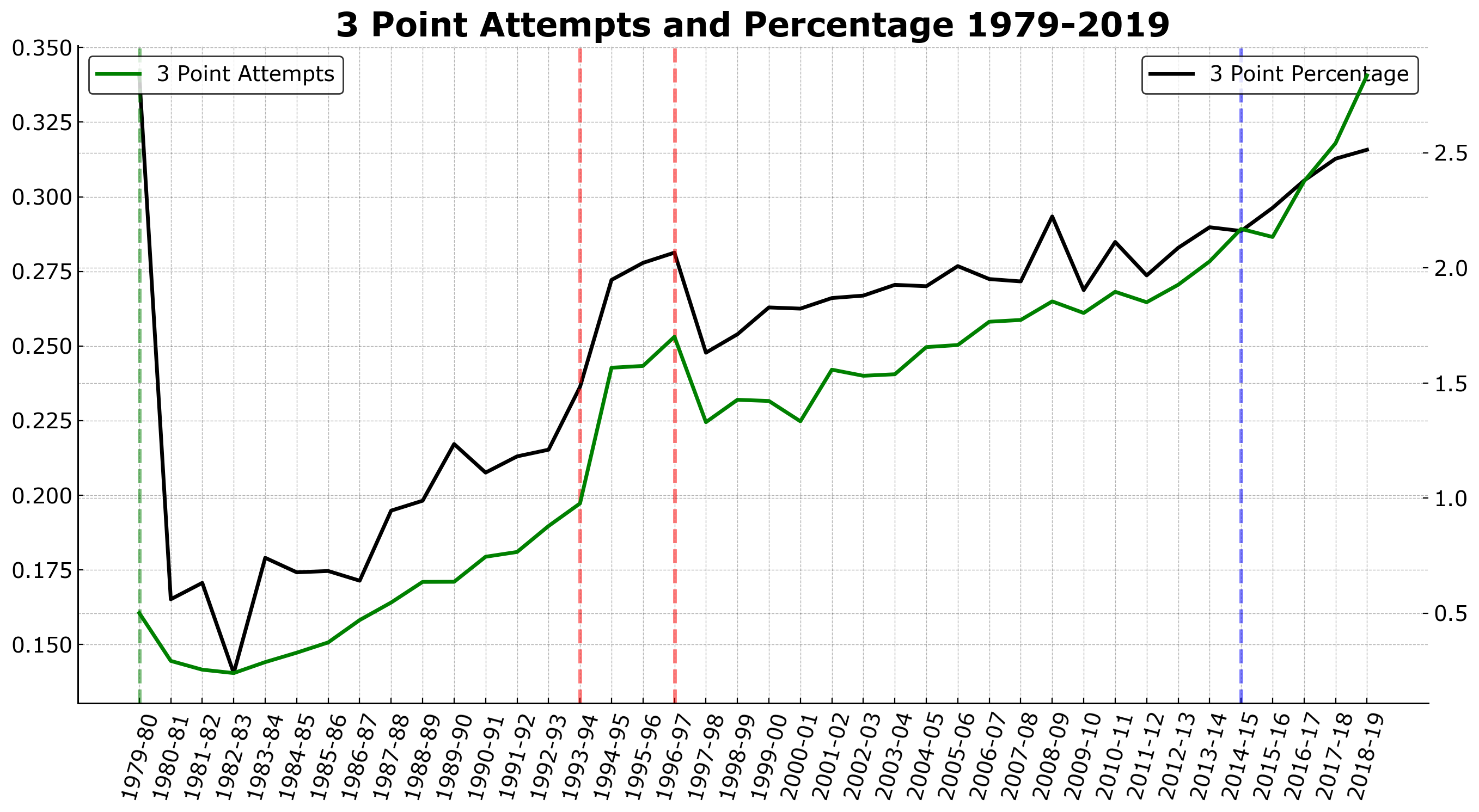
In the plot above, we can see that during the introduction of the 3 point line 1979-80 Season, 3 point accuracy was very high but this was limited to a very small sample size. The red dotted line during the 1994-95 and 1996-97 seasons indicate the 3-year period wherein the NBA shortened the 3 point line in order to increase volume and usage of the 3 pointer in the NBA game. Lastly, we can see the rapid increase in both the attempts and accuracy of the 3 pointer during the 2014-15 season onwards. This is marked by the blue dotted line that indicates the year that Steph Curry won his first MVP season and the Golden State Warriors dominated the NBA to win their first championship in 50 years. This is a turning point in the 3 point arena of the game, as most teams in the current NBA cannot survive without a good 3 point shooter, and this is reflected in the marked increase in both volume and accuracy of 3 point shooters in the league since then.
Load Data
We proceed with clustering the NBA players.
# connect to sqlite db
conn = sqlite3.connect('Lab_Lab 5_nbaDB.db')
df = pd.read_sql('SELECT * FROM season_average', conn, index_col='index')
df.head()
| Season | Age | Tm | Lg | Pos | G | GS | MP | FG | FGA | ... | ORB | DRB | TRB | AST | STL | BLK | TOV | PF | PTS | Player | |
|---|---|---|---|---|---|---|---|---|---|---|---|---|---|---|---|---|---|---|---|---|---|
| index | |||||||||||||||||||||
| 0 | 1990-91 | 22.0 | POR | NBA | PF | 43.0 | 0.0 | 6.7 | 1.3 | 2.7 | ... | 0.6 | 1.4 | 2.1 | 0.3 | 0.1 | 0.3 | 0.5 | 0.9 | 3.1 | Alaa Abdelnaby |
| 1 | 1991-92 | 23.0 | POR | NBA | PF | 71.0 | 1.0 | 13.2 | 2.5 | 5.1 | ... | 1.1 | 2.5 | 3.7 | 0.4 | 0.4 | 0.2 | 0.9 | 1.9 | 6.1 | Alaa Abdelnaby |
| 2 | 1992-93 | 24.0 | TOT | NBA | PF | 75.0 | 52.0 | 17.5 | 3.3 | 6.3 | ... | 1.7 | 2.8 | 4.5 | 0.4 | 0.3 | 0.3 | 1.3 | 2.5 | 7.7 | Alaa Abdelnaby |
| 3 | 1992-93 | 24.0 | MIL | NBA | PF | 12.0 | 0.0 | 13.3 | 2.2 | 4.7 | ... | 1.0 | 2.1 | 3.1 | 0.8 | 0.5 | 0.3 | 1.1 | 2.0 | 5.3 | Alaa Abdelnaby |
| 4 | 1992-93 | 24.0 | BOS | NBA | PF | 63.0 | 52.0 | 18.3 | 3.5 | 6.6 | ... | 1.8 | 3.0 | 4.8 | 0.3 | 0.3 | 0.3 | 1.3 | 2.6 | 8.2 | Alaa Abdelnaby |
5 rows × 31 columns
As the collected data for seasons are written in the NBA format of yyyy-yy, we create a function named get_year in order to create a new column that contains the ending year of each season i.e., 2008-09 will become 2009.
def get_year(x):
    year = re.search('\d+$', x).group(0)
    year = int(year)

    if year < 20:
        year += 2000
    else:
        year += 1900

    return year
As we are interested in seeing the progression of the NBA players for the last 10 years (2009-2019), we filter our dataframe to exclude all the years before the 2009 season. The resulting dataframe contains null values and non-numeric values i.e., “Did not play”, which we remove by dropping these rows. Lastly, we slice our final dataframe columns to include only the columns that are not correlated as shown in the heatmap discussed previously.
df['year'] = df.Season.apply(get_year)
df2 = df[df.year>=2009].drop('Season', axis=1)
df2.shape
(7092, 31)
df3 = df2.drop_duplicates(subset=['Player', 'year'])
df3 = df3.sort_values(['Player', 'year']).reset_index(drop=True)
print(df3.shape)
df3.head(2)
(5550, 31)
| Age | Tm | Lg | Pos | G | GS | MP | FG | FGA | FG% | ... | DRB | TRB | AST | STL | BLK | TOV | PF | PTS | Player | year | |
|---|---|---|---|---|---|---|---|---|---|---|---|---|---|---|---|---|---|---|---|---|---|
| 0 | 24.0 | DAL | NBA | C | 22 | 0 | 7.4 | 0.8 | 1.9 | 0.405 | ... | 1.3 | 1.6 | 0.2 | 0.0 | 0.6 | 0.5 | 1.0 | 2.2 | A.J. Hammons | 2017 |
| 1 | 23.0 | IND | NBA | PG | 56.0 | 2.0 | 15.4 | 2.6 | 6.3 | 0.41 | ... | 1.4 | 1.6 | 1.9 | 0.6 | 0.1 | 1.1 | 0.9 | 7.3 | A.J. Price | 2010 |
2 rows × 31 columns
df3.columns
['Age', 'Pos', 'GS', 'MP', 'FG', 'TOV', 'PTS']
Index(['Age', 'Tm', 'Lg', 'Pos', 'G', 'GS', 'MP', 'FG', 'FGA', 'FG%', '3P',
       '3PA', '3P%', '2P', '2PA', '2P%', 'eFG%', 'FT', 'FTA', 'FT%', 'ORB',
       'DRB', 'TRB', 'AST', 'STL', 'BLK', 'TOV', 'PF', 'PTS', 'Player',
       'year'],
      dtype='object')
df4 = df3[df3['G'].apply(lambda x: x.replace('.', '').isnumeric())]
df4 = df4[['Player', 'year', 'G', '3P', '3P%', '2P', '2P%', 'FT%',
                'eFG%', 'ORB', 'DRB', 'AST', 'STL', 'BLK', 'PF']]

df4.dropna(inplace=True)
print(df4.shape)
df4.head(2)
(4527, 15)
| Player | year | G | 3P | 3P% | 2P | 2P% | FT% | eFG% | ORB | DRB | AST | STL | BLK | PF | |
|---|---|---|---|---|---|---|---|---|---|---|---|---|---|---|---|
| 0 | A.J. Hammons | 2017 | 22 | 0.2 | 0.5 | 0.5 | 0.375 | 0.45 | 0.464 | 0.4 | 1.3 | 0.2 | 0.0 | 0.6 | 1.0 |
| 1 | A.J. Price | 2010 | 56.0 | 1.1 | 0.345 | 1.5 | 0.472 | 0.8 | 0.494 | 0.2 | 1.4 | 1.9 | 0.6 | 0.1 | 0.9 |
df4['Player_Unique'] = df4.Player + '_' + df4.year.astype(str)
df4.loc[:, 'G':'PF'] = df4.loc[:,'G':'PF'].astype(np.float64)
print(df4.shape)
df4.head(2)
(4527, 16)
| Player | year | G | 3P | 3P% | 2P | 2P% | FT% | eFG% | ORB | DRB | AST | STL | BLK | PF | Player_Unique | |
|---|---|---|---|---|---|---|---|---|---|---|---|---|---|---|---|---|
| 0 | A.J. Hammons | 2017 | 22.0 | 0.2 | 0.500 | 0.5 | 0.375 | 0.45 | 0.464 | 0.4 | 1.3 | 0.2 | 0.0 | 0.6 | 1.0 | A.J. Hammons_2017 |
| 1 | A.J. Price | 2010 | 56.0 | 1.1 | 0.345 | 1.5 | 0.472 | 0.80 | 0.494 | 0.2 | 1.4 | 1.9 | 0.6 | 0.1 | 0.9 | A.J. Price_2010 |
In the final dataframe, we created a new column that concatenates the player names with the season played, as there will be multiple years per player in the dataset. We are left with the following columns:
G- Number of games played3P- Number of 3 point shots made3P%- Percentage of 3 point shots made2P- Number of 2 point shots made2P%- Percentage of 2 point shots madeFT%- Percentage of free throws madeeFG%- Effective field goal percentage ((FGM + 0.5 * 3PM) / FGA)ORB- Number of Offensive ReboundsDRB- Number of Defensive ReboundsAST- Number of assistsSTL- Number of stealsBLK- Number of blocksPF- Number of personal fouls
Total number of features: 13.
Dimensionality Reduction (PCA)
As we are still left with 13 features, we perform dimensionality reduction using Principal Component Analysis. Using PCA, we transform the dataset on to the vectors that have the most explained variance. As such, each principal component in the analysis is not representative of a feature, but rather, a combination of all features that are weighted. In doing so, we are able to reduce the number of “features” that we will be using for the analysis, thereby reducing the amount of noise in the model.
However, before proceeding to Principal Component Analysis, we must first ensure that the dataset is mean-centered at 0 as this is one of the pre-requisites of PCA. We can achieve this by using the StandardScaler function from sklearn.preprocessing. This function scales all the features in order to have a new mean centered at 0.
X = df4.iloc[:,2:-1]
scaler = StandardScaler()
X_scaled = scaler.fit_transform(X)
Once we have scaled the dataset, we take a look at the directions of each of the vectors that represent a feature in our data. This will give us a better idea in terms of the directionality or relationship of each feature with each other. In the plot below, we show the direction of each feature vector (red arrow) on the plot of the first 2 principal components.
V = np.cov(X_scaled, rowvar=False)
lambdas, w = np.linalg.eig(V)
indices = np.argsort(lambdas)[::-1]
lambdas = lambdas[indices]
w = w[:, indices]
new_X = np.dot(X_scaled, w)
fig, ax = plt.subplots(dpi=120)
ax.scatter(new_X[:,0], new_X[:,1])
for feat, feat_name in zip(w, df4.columns[2:-1]):
    ax.arrow(0, 0, 7*feat[0], 7*feat[1], color='r', width=0.1, ec='none')
    ax.text(7*feat[0], 7*feat[1], feat_name, ha='center', color='k')
ax.set_xlabel('PC1')
ax.set_ylabel('PC2')
ax.set_title('Plot of Eigenvectors against first 2 PCs');
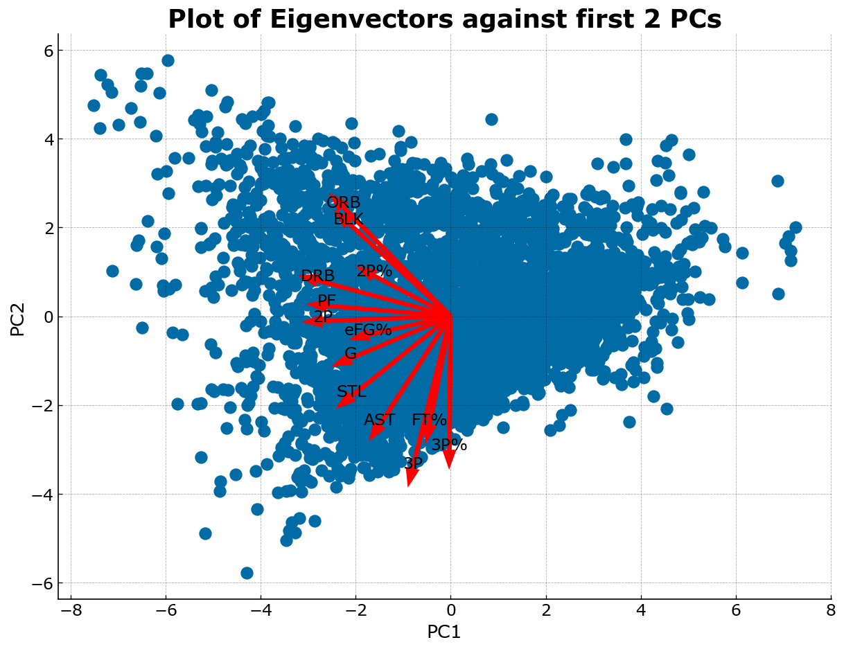
In the plot of the feature vectors above, we can see that there are relationships among the feature vectors that are of interest in the context of an NBA game:
- The 3 point shooting vector (as indicated by
3Pand3P%) is almost opposite to the feature vector for offensive rebounds and blocks (as indicated byORBandBLK). In the context of an NBA game, this makes sense as a player who shoots three pointers would most likely be positioned outside of the 3 point line, thus giving him a disadvantage on offensive rebounds due to the distance from the basket. This accounts for the negative relationship between these two vectors. - In the same vein, 2 point shooting is correlated with defensive rebounds, personal fouls, and effective field goal percentage (as indicated by
DRB,PF, andeFG%, respectively). This is most likely due to the “inside play” during NBA games, and can be seen the most among centers and power forwards as these positions are typically played near the paint. This proximity to the rim accounts for their high effective field goal percentage, propensity for defensive rebounds, and their prevalence of 2 point shots. As these players are also the ones most likely to be inside the paint, they are correlated with personal fouls as well as they are tasked with defending the rim from opponents, thus running straight into the line of fire of driving opponents and increasing their probability of committing a foul. - An interesting observation is that that in the traditional positions of the NBA, we can see a separation along the vector of
eFG%wherein all the vectors above it (2P,PF,DRB,2P%,ORB, andBLK) are traditionally attributes of Centers and Forwards, or the “inside” players. Whereas the vectors opposite of this group (G,STL,AST,FT%,3P,3P%) are traditionally attributed more toward guards who are the “outside” players and ball handlers of the game.
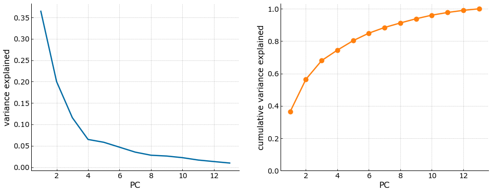
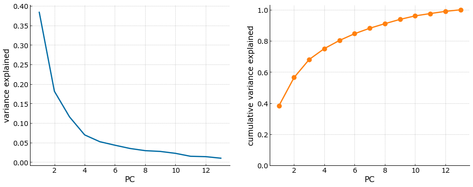
A main advantage of PCA is being able to limit the number of features that we use to describe the dataset. To achieve this, we will need to limit the original features by setting a target percentage (%) of explained variance that we want to retain using the lowest number of principal components. The functions below convert our scaled numpy array into the principal components and remove those principal components that are beyond our target explained variance of 80%. This leaves us with 5 principal components as can be seen in the cumulative variance explained plot below.
def get_min_pcs(X, var):
    colors = plt.rcParams["axes.prop_cycle"].by_key()["color"]
    pca = PCA(svd_solver='full')
    new_X2 = pca.fit_transform(X)

    var_explained = pca.explained_variance_ratio_

    fig, ax = plt.subplots(1, 2, figsize=(16,6))
    ax[0].plot(np.arange(1, len(var_explained)+1), var_explained, c=colors[0])
    ax[0].set_xlabel('PC')
    ax[0].set_ylabel('variance explained')

    cum_var_explained = var_explained.cumsum()
    ax[1].plot(np.arange(1, len(cum_var_explained)+1),
                  cum_var_explained, '-o', c=colors[1])
    ax[1].set_ylim(bottom=0)
    ax[1].set_xlabel('PC')
    ax[1].set_ylabel('cumulative variance explained');

    return new_X2, np.searchsorted(cum_var_explained, var) + 1

def project(X_rotated, min_pcs):
    pca = PCA(n_components=min_pcs, svd_solver='full')
    X_new = pca.fit_transform(X_rotated)
    return X_new
X_rotated, min_pcs = get_min_pcs(X_scaled, 0.8)
X_new = project(X_rotated, min_pcs)
Clustering Model (K-Means)
Once we have reduced the dimensionality of the data, we can proceed with the clustering. The method for clustering chosen for this data is KMeans clustering. This works by assigning a random “mean point” in the data and adjusts each point by getting the closest points to the initally assigned mean point. The algorithm iterates this through multiple cycles, adjusting the mean point of each formed cluster until there are no more changes in the assigned mean point of each cluster.
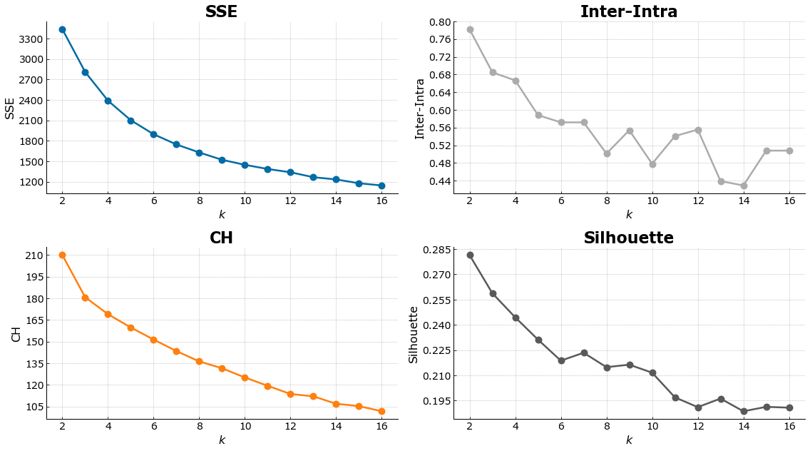
A prerequisite of the KMeans algorithm is that we will need to provide a number of clusters to use. In order to select the optimal number of clusters, we run an iteration of KMeans for k=2 until k=16 and plot the various internal validation criteria:
- SSE(Sum of Squares Error)
- Inter-Intra Cluster Range
- Calinski-Harabasz
- Silhouette Coefficient
kmeans_nba = KMeans(random_state=1337)
out = cluster_range(X_new, kmeans_nba, 16, actual=None)
plot_internal(out['inertias'], out['chs'], out['iidrs'], out['scs']);
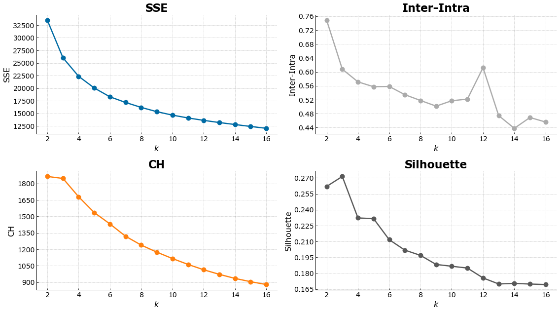
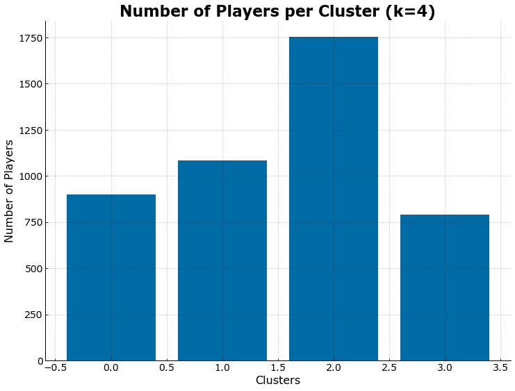
The optimal number of k chosen is 4. This number is at the elbow point of the SSE and Inter-Intra cluster range, as well as retaining a high CH score, and Silhouette Coefficient. We proceed with clustering the data using KMeans with an optimal number of 4 clusters as its hyperparameter.
# number of clusters
clusters = 4
y_predicted = out['ys'][clusters-2]

df4['y_predicted'] = y_predicted
len_clusters = []
for n in set(y_predicted):
    c = df4.loc[y_predicted==n]
    cluster_count = len(c)
    len_clusters.append(cluster_count)
fig, ax = plt.subplots()
ax.bar(Counter(y_predicted).keys(), Counter(y_predicted).values())
ax.set_ylabel('Number of Players')
ax.set_xlabel('Clusters')
ax.set_title('Number of Players per Cluster (k=4)');
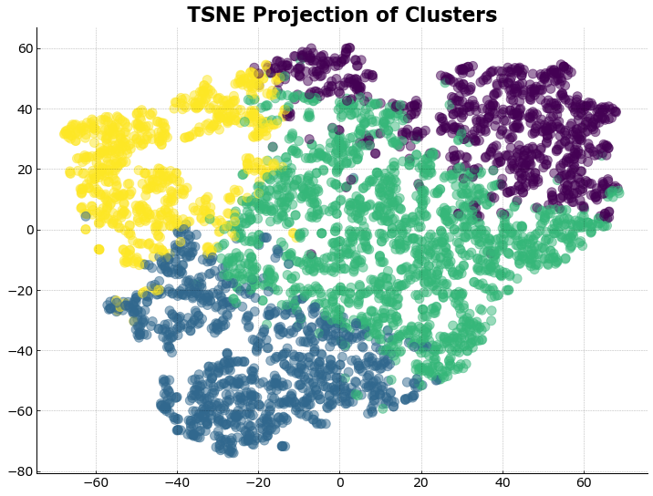
X_players_new = TSNE(n_components=2,random_state=1337).fit_transform(X_new)
fig, ax = plt.subplots()
ax.scatter(X_players_new[:,0], X_players_new[:,1], c=list(y_predicted),
           alpha=0.5)
ax.set_title('TSNE Projection of Clusters');
player_clusters = []
for i in range(clusters):
    grp = df4[df4.y_predicted==i]['Player'].to_list()
    player_clusters.append(dict(Counter(grp).most_common()))
Analysis
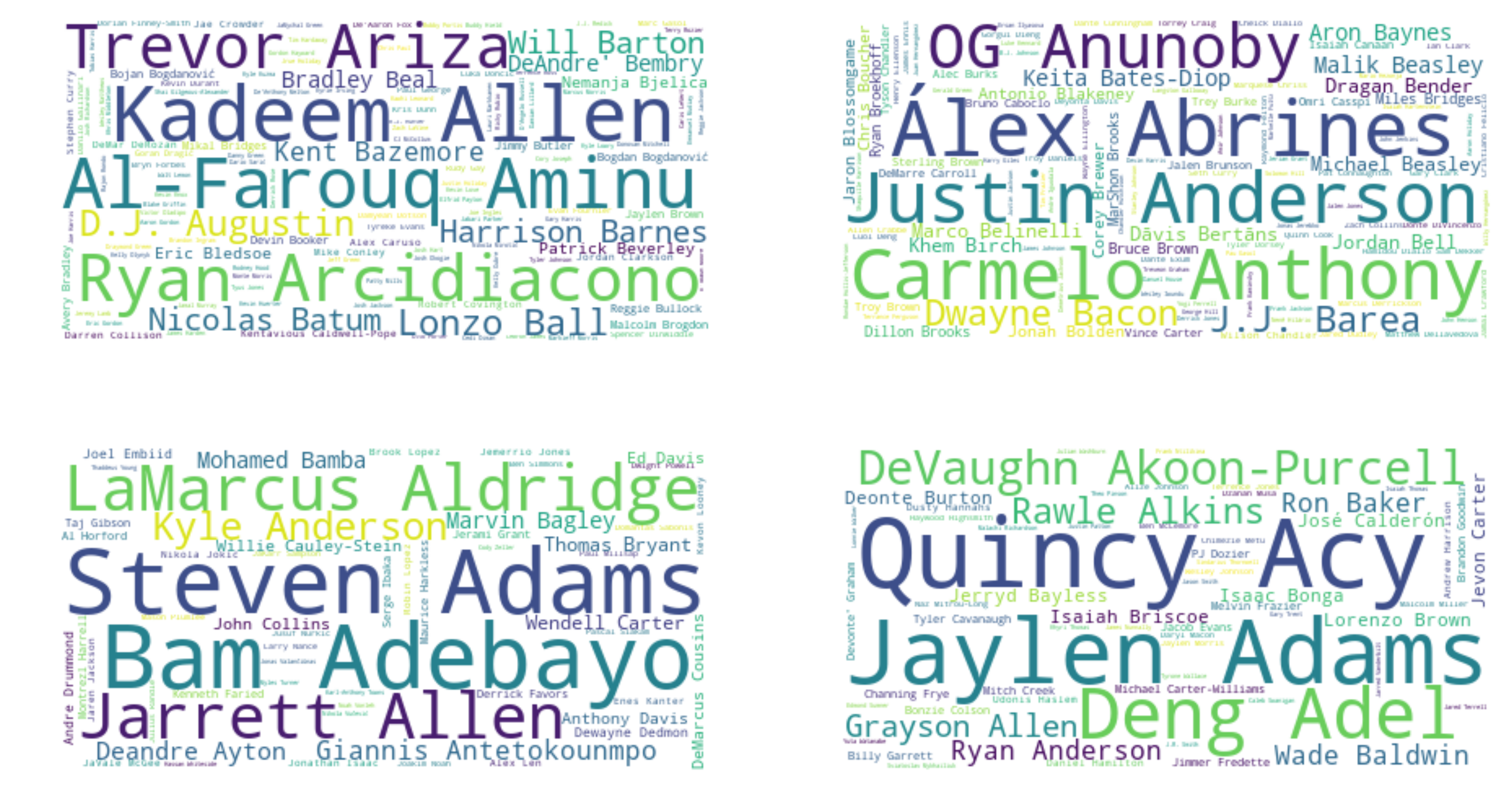
Once we have clustered our player data, we first take a look at the player composition of each cluster. To get an overview of the players per cluster, we plot the names of the players in a word cloud.
fig, axs = plt.subplots(2,2, figsize=(16,9))
for i, ax in enumerate(fig.axes):
    freq = player_clusters[i]
    wordcloud_obj = WordCloud(background_color="white",
                              mask=None,
                              contour_width=1,
                              contour_color='white',
                              random_state=2018)
    wordcloud = wordcloud_obj.generate_from_frequencies(frequencies=freq)

    # Display the generated image
    ax.imshow(wordcloud, interpolation='bilinear')
    ax.axis("off")
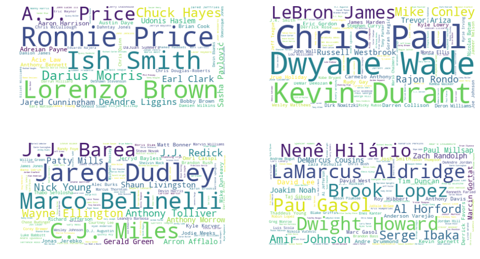
From the cursory view given by the wordclouds, we can immediately see two distinct clusters: star players and centers. These are the clusters on the right hand side as denoted by the star cluster of Chris Paul, Dwyane Wade, Kevin Durant, and Lebron James, and the cluster of centers/bigs as denoted by LaMarcus Aldridge, Brook Lopez, Dwight Howard, Pau Gasol, and others. The other two clusters seem to be a mix of guards and forwards that are perhaps clustered based on their skill level as the cluster with Jared Dudley, J.J. Barea, C.J. Miles and others are known bench players or 6th man players for different teams. To get a clearer picture of the description per cluster, we can take a look at their average stats per player.
df5 = df4.merge(df3[['Player', 'year', 'Age', 'Pos',
                    'GS', 'MP', 'FG', 'TOV', 'PTS']], on=['Player', 'year'])
df5[df5.columns[-5:]] = df5[df5.columns[-5:]].astype(float)
df5.groupby('y_predicted')[df5.columns[2:]].mean().transpose()
| y_predicted | 0 | 1 | 2 | 3 |
|---|---|---|---|---|
| G | 29.056604 | 69.080184 | 57.284817 | 67.415716 |
| 3P | 0.268257 | 1.469401 | 0.831792 | 0.185044 |
| 3P% | 0.216518 | 0.355161 | 0.348482 | 0.163632 |
| 2P | 0.947503 | 4.079816 | 1.734418 | 4.375792 |
| 2P% | 0.404438 | 0.480169 | 0.484890 | 0.527292 |
| FT% | 0.670225 | 0.800956 | 0.767463 | 0.693532 |
| eFG% | 0.402485 | 0.502191 | 0.507717 | 0.522745 |
| ORB | 0.419645 | 0.808756 | 0.573916 | 2.180608 |
| DRB | 1.235738 | 3.544700 | 2.069121 | 4.950824 |
| AST | 0.950166 | 4.185899 | 1.461016 | 1.582890 |
| STL | 0.351387 | 1.171060 | 0.551142 | 0.730545 |
| BLK | 0.158713 | 0.373548 | 0.258048 | 1.012928 |
| PF | 1.083685 | 2.201290 | 1.600514 | 2.556907 |
| y_predicted | 0.000000 | 1.000000 | 2.000000 | 3.000000 |
| Age | 25.726970 | 26.663594 | 26.769406 | 26.250951 |
| GS | 2.593785 | 55.860829 | 14.947489 | 45.475285 |
| MP | 11.117203 | 31.570968 | 18.800400 | 26.051838 |
| FG | 1.214650 | 5.545438 | 2.567009 | 4.561090 |
| TOV | 0.619867 | 2.091705 | 0.899144 | 1.483777 |
| PTS | 3.258713 | 15.398894 | 6.966781 | 11.452091 |
positions = []
for i in set(y_predicted):
    positions.append(dict(Counter(df5[df5['y_predicted'] == i]['Pos'])))
pd.DataFrame.from_records(positions).fillna(0)[['C', 'PF', 'SF', 'SG', 'PG']]
| C | PF | SF | SG | PG | |
|---|---|---|---|---|---|
| 0 | 78 | 151 | 189 | 235 | 226 |
| 1 | 17 | 111 | 224 | 305 | 411 |
| 2 | 120 | 302 | 449 | 517 | 330 |
| 3 | 425 | 303 | 44 | 7 | 3 |
By looking at the average stats per cluster, we are able to ascertain different insights from each cluster. As mentioned previously, there is the presence of the star cluster and the centers cluster. Based on these stats, we can describe each cluster as such:
- Cluster 0 - bench players. These are players with low overall stats, the most telling of which is the number of games played in the cluster, being just about half the number of games played compared to the other clusters. This also reflects in the amount of two pointers and three pointers that they’ve made as well as the comparatively low numbers they have in the other measures. This cluster may also be the rookies or new players in the league as they have the lowest average age of all clusters.
- Cluster 1 - star players. These are the players who play the most minutes, indicating that they are the go-to guys of the team. This cluster also has the highest average stats in almost all categories, with a highlight being the number of games started, minute played, points, assists, and turnovers. The turnover rate in this cluster may be related to the number of minutes played, as well as the fact that star players usually have the ball in their hands the most while facing the stiffest defenses. The age of the players in this cluster is also telling as the average age is at around 26.66 years old, and the accepted “prime years” of an NBA player would coincide with this age range of about 26-30 years old. This cluster is predominantly made up of small forwards, shooting guards, and point guards, which coincide with the highest volume shooters in the league and make up the high scoring rate and shooting accuracy of this cluster.
- Cluster 2 - role players. These players form the role players in the team. While their numbers are better than those of cluster 0, there is a marked difference between them and the “elite” players in the league. Their numbers are generally lower than those of cluster 1 and cluster 3. Going back to the word cloud, we can see that the names of these players are composed mostly of bench players and starters who are role players, generally these are the players that you build around star players.
- Cluster 3 - big men. This cluster is predominantly composed of centers or big men as evidenced by the number of cneters and power forwards in the positions. As each team needs to start a center in the game, this role is usually very well defined in their stats such as high amount of rebounds and blocks, as well as a higher number of minutes played and highest personal fouls, as they are tasked with defending the rim from the driving opponents, making them more prone to fouling. As we saw in the feature vectors of the principal components above, this is a very well defined cluster as the feature vectors relating to big men/centers are all related or pointing in the same direction. As we expect from the PCA plot, this cluster is defined by the number of rebounds, personal fouls, and 2 pointers and 2 point accuracy.
Based on the clusters that were formed, the unsupervised KMeans algorithm seemed to cluster the players based on their skill set and skill level. Whereas we had truly elite guards/forwards in cluster 1, we also had the newbies or bench players in cluster 0. We also found that there is a concenctration of big men in cluster 3, possibly because of the strength of the feature vectors along this principal component. Thus, we deem that the clustering algorithm was able to cluster players based on both their skill set (usually related to their position or what they are able to bring to the game), and the level at which they execute at this skill set (given by the average stats for each cluster).
One of the insights we can garner from this analysis is that there is a chance that there are players that can be found in multiple clusters throughout their careers. This could be the player trajectory of starting out as a role player or bench player and eventually moving into the role of a star player during their prime years. Another possible career trajectory for this time period is that of a player coming down from their peak and being relegated into the role of a bench player or supporting player. In our clustering, the first scenario would indicate a move for players from cluster 2 into cluster 1, and the second scenario would involve a move from cluster 1 to cluster 2 or possibly cluster 0. In the past 10 years, there would be several players who fall into these categories: Klay Thompson was drafted in 2011 and played a minor role in the Golden State Warriors until their breakthrough season in 2014-2015 where he became a star player, Draymond Green similarly was drafted by GSW in 2012 and played a minor role up until the same season, and Kawhi Leonard was drafted in 2011 and played a minor role until the San Antonio Spurs won the championship in 2014 with which he won the Finals MVP award. We expect these players’ career trajectories to place them in multiple clusters in our analysis.
players0 = set(df4[df4['y_predicted']==0]['Player'].to_list())
players1 = set(df4[df4['y_predicted']==1]['Player'].to_list())
players2 = set(df4[df4['y_predicted']==2]['Player'].to_list())
players3 = set(df4[df4['y_predicted']==3]['Player'].to_list())

player_analysis = ['Klay Thompson', 'Draymond Green', 'Kawhi Leonard']
compiler = []
for j in [players0, players1, players2, players3]:
    player_dict = dict(zip(player_analysis, [""] * 3))
    for i in player_analysis:
        player_dict[i] = i in j
    compiler.append(player_dict)
pd.DataFrame.from_records(compiler, columns=player_analysis)
| Klay Thompson | Draymond Green | Kawhi Leonard | |
|---|---|---|---|
| 0 | False | True | False |
| 1 | True | True | True |
| 2 | True | False | True |
| 3 | False | False | False |
From the table above, we can see that all three of these players had different years in their career. Kawhi Leonard and Klay Thompson, both first round draft picks (15th and 11th, respectively) were most likely clustered first in cluster 2 as role players during the first half of their career, whereas Draymond Green, a second round draft pick, was first in the cluster 0 as a bench player. However, during their latter years, the three of them developed into full-fledged star players and being clustered into cluster 1 as star players for their team. We validate this by looking into the years in which each player were clustered into clusters 0, 1, and 2.
for i in ['Klay Thompson', 'Kawhi Leonard']:
    print(f'{i}:')
    print(f'Cluster 2: {df4[(df4["y_predicted"]==2) & (df4["Player"]==i)]["Player_Unique"].to_list()}')
    print(f'Cluster 1: {df4[(df4["y_predicted"]==1) & (df4["Player"]==i)]["Player_Unique"].to_list()}')
    print('\n')

d = 'Draymond Green'
print(f'{d}:')
print(f'Cluster 0: {df4[(df4["y_predicted"]==0) & (df4["Player"]==d)]["Player_Unique"].to_list()}')
print(f'Cluster 1: {df4[(df4["y_predicted"]==1) & (df4["Player"]==d)]["Player_Unique"].to_list()}')
print('\n')
Klay Thompson:
Cluster 2: ['Klay Thompson_2012']
Cluster 1: ['Klay Thompson_2013', 'Klay Thompson_2014', 'Klay Thompson_2015', 'Klay Thompson_2016', 'Klay Thompson_2017', 'Klay Thompson_2018', 'Klay Thompson_2019']


Kawhi Leonard:
Cluster 2: ['Kawhi Leonard_2012']
Cluster 1: ['Kawhi Leonard_2013', 'Kawhi Leonard_2014', 'Kawhi Leonard_2015', 'Kawhi Leonard_2016', 'Kawhi Leonard_2017', 'Kawhi Leonard_2018', 'Kawhi Leonard_2019']


Draymond Green:
Cluster 0: ['Draymond Green_2013']
Cluster 1: ['Draymond Green_2014', 'Draymond Green_2015', 'Draymond Green_2016', 'Draymond Green_2017', 'Draymond Green_2018', 'Draymond Green_2019']
From the list above, we can see that the career trajectories of Klay Thompson and Kawhi Leonard mirror each other down to the year that they entered and their rookie years serving as a role player before transitioning into elite status on their second year. Similarly, Draymond Green spent his first year as a bench player before breaking out as an elite star player in his second year.
2019 NBA Players
After clustering the NBA players for the 10 year period between 2009-2019, we take a look at the most recent NBA season and cluster the players for this year to validate whether or not these clusters have changed.
df2019 = df[df['year'] == 2019]
df2019.drop_duplicates(['Player', 'year'], keep='first', inplace=True)
df2019 = df2019.reset_index()
df2019_players = df2019['Player']
df2019 = df2019[['Player', 'year', 'G', '3P', '3P%', '2P', '2P%', 'FT%',
                'eFG%', 'ORB', 'DRB', 'AST', 'STL', 'BLK', 'PF']]
df2019 = df2019[~df2019['G'].str.contains('Did')]
df2019.dropna(how='any', inplace=True)
df2019[df2019['Player'].str.contains('Ray')]
| Player | year | G | 3P | 3P% | 2P | 2P% | FT% | eFG% | ORB | DRB | AST | STL | BLK | PF | |
|---|---|---|---|---|---|---|---|---|---|---|---|---|---|---|---|
| 164 | Raymond Felton | 2019 | 33.0 | 0.6 | 0.328 | 1.1 | 0.473 | 0.923 | 0.481 | 0.1 | 0.9 | 1.6 | 0.3 | 0.2 | 0.9 |
| 458 | Ray Spalding | 2019 | 14.0 | 0.0 | 0.0 | 1.8 | 0.568 | 0.333 | 0.532 | 1.1 | 2.4 | 0.4 | 0.6 | 0.6 | 1.6 |
PCA 2019
X2019_scaled = scaler.fit_transform(df2019[df2019.columns[2:]])
X2019_rotated, min_pcs2019 = get_min_pcs(X2019_scaled, 0.8)
X2019_new = project(X2019_rotated, min_pcs2019)
In clustering the 2019 stats, we do dimensionality reduction through Principal Component Analysis in order to get the nuumber of PCs that will explain 80% of our total explained variance. This is similar to the one for the aggregated 10 year player cluster as we will be using 5 principal components.
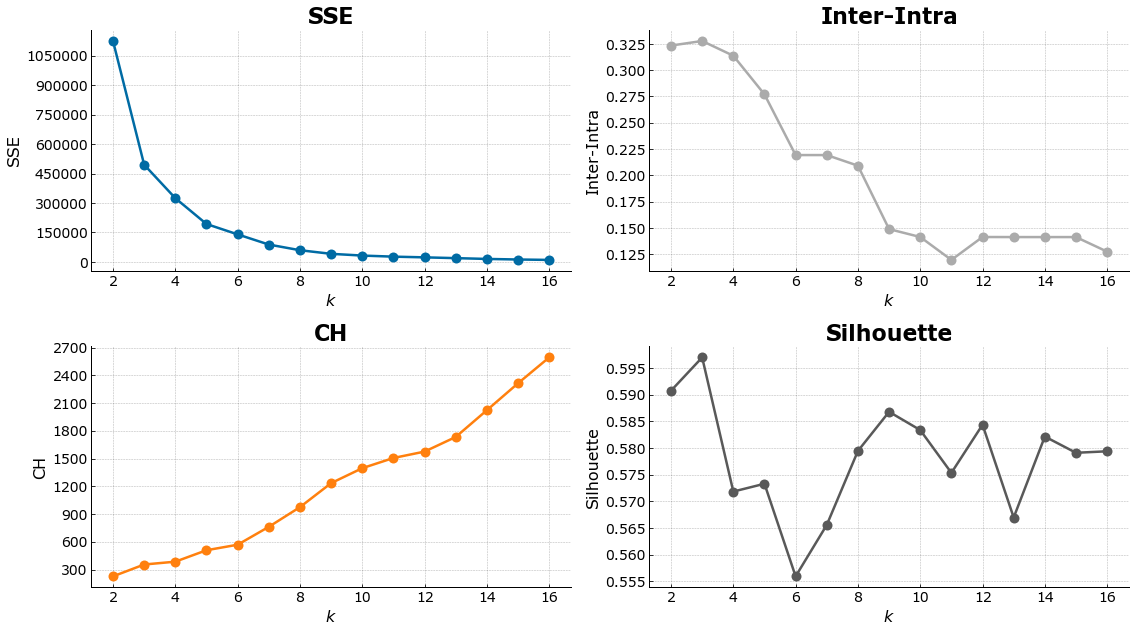
KMeans 2019
kmeans_nba2019 = KMeans(random_state=1337)
out = cluster_range(X2019_new, kmeans_nba2019, 16, actual=None)
plot_internal(out['inertias'], out['chs'], out['iidrs'], out['scs']);
# number of clusters
clusters = 4
y_predicted = out['ys'][clusters-2]

df2019['y_predicted'] = y_predicted
len_clusters = []
for n in set(y_predicted):
    c = df2019.loc[y_predicted==n]
    cluster_count = len(c)
    len_clusters.append(cluster_count)
len_clusters
[146, 210, 56, 63]
player_clusters = []
for i in range(clusters):
    grp = df2019[df2019.y_predicted==i]['Player'].to_list()
    player_clusters.append(dict(Counter(grp).most_common()))
Analysis 2019
fig, axs = plt.subplots(2,2, figsize=(16,9), dpi=300)
for i, ax in enumerate(fig.axes):
    freq = player_clusters[i]
    wordcloud_obj = WordCloud(background_color="white",
                              mask=None,
                              contour_width=1,
                              contour_color='white',
                              random_state=2018)
    wordcloud = wordcloud_obj.generate_from_frequencies(frequencies=freq)

    # Display the generated image
    ax.imshow(wordcloud, interpolation='bilinear')
    ax.axis("off")
df2019[df2019.columns[2:-1]] = df2019[df2019.columns[2:-1]].astype(float)
grouped = df2019.merge(df3[['Player', 'year', 'Age', 'Pos',
                    'GS', 'MP', 'FG', 'TOV', 'PTS']], on=['Player', 'year'])
grouped[grouped.columns[-5:]] = grouped[grouped.columns[-5:]].astype(float)
grouped.groupby('y_predicted')[grouped.columns[2:]].mean().transpose()
| y_predicted | 0 | 1 | 2 | 3 |
|---|---|---|---|---|
| G | 67.527397 | 48.119048 | 66.785714 | 20.619048 |
| 3P | 1.734247 | 0.736190 | 0.532143 | 0.341270 |
| 3P% | 0.360445 | 0.314329 | 0.266179 | 0.223016 |
| 2P | 3.584247 | 1.494286 | 4.810714 | 0.734921 |
| 2P% | 0.494103 | 0.520929 | 0.575821 | 0.407683 |
| FT% | 0.793096 | 0.729205 | 0.711804 | 0.674730 |
| eFG% | 0.514411 | 0.522633 | 0.561929 | 0.388841 |
| ORB | 0.789726 | 0.616190 | 2.312500 | 0.296825 |
| DRB | 3.704110 | 2.073333 | 5.687500 | 1.112698 |
| AST | 3.690411 | 1.246667 | 2.221429 | 0.953968 |
| STL | 1.021233 | 0.447143 | 0.841071 | 0.304762 |
| BLK | 0.395205 | 0.281429 | 1.101786 | 0.112698 |
| PF | 2.203425 | 1.547143 | 2.701786 | 0.936508 |
| y_predicted | 0.000000 | 1.000000 | 2.000000 | 3.000000 |
| Age | 26.493151 | 26.214286 | 25.392857 | 24.603175 |
| GS | 50.020548 | 8.004762 | 49.125000 | 1.301587 |
| MP | 29.271918 | 15.933810 | 26.544643 | 9.588889 |
| FG | 5.315753 | 2.232381 | 5.341071 | 1.073016 |
| TOV | 1.806849 | 0.721905 | 1.608929 | 0.509524 |
| PTS | 14.733562 | 6.013810 | 13.685714 | 2.942857 |
When we cluster all the players for just one year, we can see that there are roughly the same clusters as in the aggregate clustering. There are still clusters for the following:
- Big men/Defensive - Cluster 2. These are players that lead all clusters in rebounding and shot blocking as was in the aggregate clustering.
- Elite/Stars - Cluster 0. These are the star players who play the most minutes and score the most points.
- Bench Players - Cluster 3. These are the players with the lowest games played and overall stats. Similar to the aggregate clusters, these are developing players or rookies, as evident with their low average age.
- Role Players - Cluster 1. These players are the role players for every team. Similar again to the aggregate clustering, we see that they are relatively balanced in their stats and can contribute in many ways.
Clustering 3 Point Shooters
As we’ve seen in the EDA section, there has been a growing trend of 3 point shooting in the league, led by the teams of Steph Curry and James Harden. In this section, we look to cluster the 3 point shooters in the league to see what differentiates them from one another. In the selection of players to cluster, we limited these to the players who have attempted at least 200 3 point shots throughout the course of the season, which is the basis for candidacy for the 3 point shooting crown of the NBA. We are left with 158 players after filtering for this criteria.
df6 = pd.read_sql('''SELECT * FROM shot_finder''', conn)
df6[df6.columns[4:]] = df6[df6.columns[4:]].astype(float)
df6 = df6[df6['3PA'] > 200]
df7 = df6[['3PA', '3P%', "%Ast'd"]]
To be able to filter out the elite 3 point shooters in the league, we will be looking at three factors: the volume of shots, accuracy of their shots, and the percentage of shots they can create on their own. These stats correspond to 3PA, 3P%, and %Ast'd, respectively and reflect the three biggest factors that are relevant in the NBA today: the number, accuracy, and skill in creating and making 3 point shots. At the end of this clustering analysis, we will be able to bucket the different kind of three point shooters in the league.
As there are only 3 features to be used, we will forego the Principal Component Analysis section and go straight to clustering these players.
kmeans_3p = KMeans(random_state=1337)
out = cluster_range(df7.to_numpy(), kmeans_3p, 16, actual=None)
plot_internal(out['inertias'], out['chs'], out['iidrs'], out['scs']);
Based on the internal validation criteria above, we select 6 as the optimal number of clusters. This is chosen as the elbow point of the inter-intra cluster range and SSE, as well as maintaining a high silhouette score (although the difference between the max and min Silhouette score is only ~0.5).
# number of clusters
clusters3p = 6
y_predicted3p = out['ys'][clusters3p-2]

df6['y_predicted'] = y_predicted3p
print('Average Player Stats per Cluster:')
df6.groupby('y_predicted')[['3PA', '3P%', "%Ast'd"]].mean().transpose()
Average Player Stats per Cluster:
| y_predicted | 0 | 1 | 2 | 3 | 4 | 5 |
|---|---|---|---|---|---|---|
| 3PA | 653.909091 | 378.472222 | 229.42000 | 465.083333 | 1028.000 | 305.25000 |
| 3P% | 0.385182 | 0.371667 | 0.35136 | 0.358000 | 0.368 | 0.36225 |
| %Ast'd | 0.714091 | 0.818750 | 0.87790 | 0.769167 | 0.161 | 0.84625 |
print('Count of players per cluster:')
df6.groupby('y_predicted')[['3PA']].count().transpose()
Count of players per cluster:
| y_predicted | 0 | 1 | 2 | 3 | 4 | 5 |
|---|---|---|---|---|---|---|
| 3PA | 11 | 36 | 50 | 24 | 1 | 36 |
The summary of each stat above shows the stark difference in the different clusters that were formed, with their being an outlier cluster in cluster 4. When we take a look at the number of players in each cluster, there is a clear outlier in the players this season with only one player belonging to cluster 4.
Based on the stats per cluster, we can see:
- Cluster 2 - spot up shooters. These are the shooters who prefer staying on the perimiter and wait for the slashers or ball handlers to pass them the ball when they are open. This is evident in the low number of attempts, and the high assist rate for their three pointers.
- Cluster 5 - mix of spot up and low volume shooters. These are players who are not traditionally purely three point shooters but can knock down the shot when called upon. Additionally, they have a high assist rate meaning that they are more likely also camped out in the perimeter but do venture out on their own.
- Cluster 1 - spot up sharpshooters. These players are mostly assisted on their 3 point makes, but also shoot them at a high accuracy. As shown by their stats, they do not tend to shoot a lot of 3 pointers but are confident when they do.
For clusters 0, 3, and 4, we look into the breakdown of players per cluster to get a better understanding of the composition of each.
rel_cols = ['Player', 'Tm', 'G', '3PA', '3P%', "%Ast'd"]
df6[df6['y_predicted']==3].sort_values('3PA', ascending=False)[rel_cols].head(10)
| Player | Tm | G | 3PA | 3P% | %Ast'd | |
|---|---|---|---|---|---|---|
| 426 | Blake Griffin | DET | 75.0 | 522.0 | 0.362 | 0.561 |
| 206 | Jae Crowder | UTA | 80.0 | 522.0 | 0.331 | 0.942 |
| 423 | Donovan Mitchell | UTA | 77.0 | 519.0 | 0.362 | 0.580 |
| 443 | Luka Dončić | DAL | 72.0 | 514.0 | 0.327 | 0.423 |
| 194 | Brook Lopez | MIL | 81.0 | 512.0 | 0.365 | 0.952 |
| 330 | Joe Ingles | UTA | 82.0 | 483.0 | 0.391 | 0.825 |
| 444 | Trae Young | ATL | 80.0 | 482.0 | 0.324 | 0.423 |
| 374 | Tim Hardaway | TOT | 65.0 | 477.0 | 0.340 | 0.728 |
| 412 | Khris Middleton | MIL | 77.0 | 474.0 | 0.378 | 0.603 |
| 344 | Reggie Jackson | DET | 82.0 | 471.0 | 0.369 | 0.793 |
For cluster3, we can see that these players are elite players who are able to create their own shot and this cluster is defined by 3 point shooters who are able to dribble and spot up and make their 3 pointers with high accuracy. In this cluster, we can see the great 3 point shooters in the league with the likes of Trae Young, Khris Middleton, and others.
df6[df6['y_predicted']==0].sort_values('3PA', ascending=False)[rel_cols].head()
| Player | Tm | G | 3PA | 3P% | %Ast'd | |
|---|---|---|---|---|---|---|
| 383 | Stephen Curry | GSW | 69.0 | 810.0 | 0.437 | 0.689 |
| 392 | Paul George | OKC | 77.0 | 757.0 | 0.386 | 0.671 |
| 442 | Kemba Walker | CHO | 82.0 | 731.0 | 0.356 | 0.438 |
| 319 | Buddy Hield | SAC | 82.0 | 651.0 | 0.427 | 0.842 |
| 439 | Damian Lillard | POR | 80.0 | 643.0 | 0.369 | 0.460 |
In cluster0, we see the truly elite 3 point shooters in the league with star players such as Stephen Curry, Paul George, Kemba Walker, and Damian Lillard. These players are able to create their own shot and shoot at a very high volume while maintaining their accuracy. A point to note here is that Steph Curry is by far the best shooter of this cluster as he shoots more three pointers and has the highest accuracy, while still being able to create his own shots.
df6[df6['y_predicted']==4].sort_values('3PA', ascending=False).head()
| Rk | Player | Season | Tm | G | FG | FGA | FG% | FGX | 3P | 3PA | 3P% | 3PX | eFG% | Ast'd | %Ast'd | y_predicted | |
|---|---|---|---|---|---|---|---|---|---|---|---|---|---|---|---|---|---|
| 449 | 450 | James Harden | 2018-19 | HOU | 78.0 | 378.0 | 1028.0 | 0.368 | 650.0 | 378.0 | 1028.0 | 0.368 | 650.0 | 0.552 | 61.0 | 0.161 | 4 |
In cluster4, we find the true outlier of the 2018-19 NBA season in 3 pointers. James Harden not only shot the most 3 point attempts but also managed to shoot at a relatively high 36.8%, while also having the lowest assisted shot percentage which shows that he is taking most of these 3 point shots off his own dribbles. This also most likely means that these shots are contested as he would be holding the ball at the time before his shot. In this cluster, he is the only player as he is by far the player who shot the most 3’s and has the lowest assisted 3 point rate.
X_players_new3p = TSNE(n_components=2,random_state=1337).fit_transform(df7.to_numpy())
fig, ax = plt.subplots()
ax.scatter(X_players_new3p[:,0], X_players_new3p[:,1], c=list(y_predicted3p),
           alpha=0.5)
ax.set_title('TSNE Projection of Clusters');
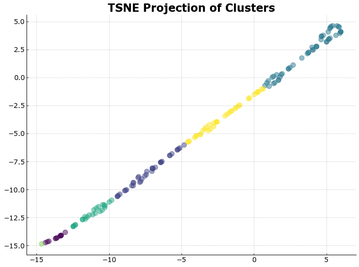
Lastly, when we plot the clusters on the tSNE representation of the dataset, we see that there is a very good separation between the clusters as there are no overlaps that can be seen. In the lower left quadrant, we see the very elite shooters, with one outlier (James Harden). In testing out the different values for k, it showed that even at different values of k, James Harden still clusters on his own as his stats are above and beyond the others for this season.
Appendix
Players per 3 Point Cluster (clusters 2, 3, 5)
Cluster 2
df6[df6['y_predicted']==2].sort_values('3PA', ascending=False).head()
| Rk | Player | Season | Tm | G | FG | FGA | FG% | FGX | 3P | 3PA | 3P% | 3PX | eFG% | Ast'd | %Ast'd | y_predicted | |
|---|---|---|---|---|---|---|---|---|---|---|---|---|---|---|---|---|---|
| 144 | 145 | Jonathan Isaac | 2018-19 | ORL | 72.0 | 86.0 | 266.0 | 0.323 | 180.0 | 86.0 | 266.0 | 0.323 | 180.0 | 0.485 | 85.0 | 0.988 | 2 |
| 224 | 225 | Garrett Temple | 2018-19 | TOT | 72.0 | 90.0 | 264.0 | 0.341 | 174.0 | 90.0 | 264.0 | 0.341 | 174.0 | 0.511 | 84.0 | 0.933 | 2 |
| 236 | 237 | Joel Embiid | 2018-19 | PHI | 61.0 | 79.0 | 263.0 | 0.300 | 184.0 | 79.0 | 263.0 | 0.300 | 184.0 | 0.451 | 73.0 | 0.924 | 2 |
| 428 | 429 | Dwyane Wade | 2018-19 | MIA | 68.0 | 86.0 | 261.0 | 0.330 | 175.0 | 86.0 | 261.0 | 0.330 | 175.0 | 0.494 | 47.0 | 0.547 | 2 |
| 190 | 191 | Tyler Johnson | 2018-19 | TOT | 56.0 | 90.0 | 260.0 | 0.346 | 170.0 | 90.0 | 260.0 | 0.346 | 170.0 | 0.519 | 86.0 | 0.956 | 2 |
Cluster 3
df6[df6['y_predicted']==3].sort_values('3PA', ascending=False).head()
| Rk | Player | Season | Tm | G | FG | FGA | FG% | FGX | 3P | 3PA | 3P% | 3PX | eFG% | Ast'd | %Ast'd | y_predicted | |
|---|---|---|---|---|---|---|---|---|---|---|---|---|---|---|---|---|---|
| 426 | 427 | Blake Griffin | 2018-19 | DET | 75.0 | 189.0 | 522.0 | 0.362 | 333.0 | 189.0 | 522.0 | 0.362 | 333.0 | 0.543 | 106.0 | 0.561 | 3 |
| 206 | 207 | Jae Crowder | 2018-19 | UTA | 80.0 | 173.0 | 522.0 | 0.331 | 349.0 | 173.0 | 522.0 | 0.331 | 349.0 | 0.497 | 163.0 | 0.942 | 3 |
| 423 | 424 | Donovan Mitchell | 2018-19 | UTA | 77.0 | 188.0 | 519.0 | 0.362 | 331.0 | 188.0 | 519.0 | 0.362 | 331.0 | 0.543 | 109.0 | 0.580 | 3 |
| 443 | 444 | Luka Dončić | 2018-19 | DAL | 72.0 | 168.0 | 514.0 | 0.327 | 346.0 | 168.0 | 514.0 | 0.327 | 346.0 | 0.490 | 71.0 | 0.423 | 3 |
| 194 | 195 | Brook Lopez | 2018-19 | MIL | 81.0 | 187.0 | 512.0 | 0.365 | 325.0 | 187.0 | 512.0 | 0.365 | 325.0 | 0.548 | 178.0 | 0.952 | 3 |
Cluster 5
df6[df6['y_predicted']==5].sort_values('3PA', ascending=False).head()
| Rk | Player | Season | Tm | G | FG | FGA | FG% | FGX | 3P | 3PA | 3P% | 3PX | eFG% | Ast'd | %Ast'd | y_predicted | |
|---|---|---|---|---|---|---|---|---|---|---|---|---|---|---|---|---|---|
| 146 | 147 | Dāvis Bertāns | 2018-19 | SAS | 76.0 | 145.0 | 338.0 | 0.429 | 193.0 | 145.0 | 338.0 | 0.429 | 193.0 | 0.643 | 143.0 | 0.986 | 5 |
| 296 | 297 | Kelly Oubre | 2018-19 | TOT | 69.0 | 108.0 | 338.0 | 0.320 | 230.0 | 108.0 | 338.0 | 0.320 | 230.0 | 0.479 | 94.0 | 0.870 | 5 |
| 369 | 370 | Terry Rozier | 2018-19 | BOS | 78.0 | 119.0 | 337.0 | 0.353 | 218.0 | 119.0 | 337.0 | 0.353 | 218.0 | 0.530 | 88.0 | 0.739 | 5 |
| 163 | 164 | Lauri Markkanen | 2018-19 | CHI | 52.0 | 120.0 | 332.0 | 0.361 | 212.0 | 120.0 | 332.0 | 0.361 | 212.0 | 0.542 | 117.0 | 0.975 | 5 |
| 272 | 273 | Malik Monk | 2018-19 | CHO | 71.0 | 109.0 | 330.0 | 0.330 | 221.0 | 109.0 | 330.0 | 0.330 | 221.0 | 0.495 | 98.0 | 0.899 | 5 |